《动手学深度学习 Pytorch版》 10.2 注意力汇聚：Nadaraya-Watson 核回归

import torch
from torch import nn
from d2l import torch as d2l

1964 年提出的 Nadaraya-Watson 核回归模型是一个简单但完整的例子，可以用于演示具有注意力机制的机器学习。

10.2.1 生成数据集

根据下面的非线性函数生成一个人工数据集，其中噪声项 $ϵ$ 服从均值为 0 ，标准差为 0.5 的正态分布：

$${\mathbf{y}}_i=2\sin {\mathbf{x}}_i+{\mathbf{x}}_i^{0.8}+ϵ$$

n_train = 50  # 训练样本数
x_train, _ = torch.sort(torch.rand(n_train) * 5)   # 排序后的训练样本

def f(x):
    return 2 * torch.sin(x) + x**0.8

y_train = f(x_train) + torch.normal(0.0, 0.5, (n_train,))  # 训练样本的输出
x_test = torch.arange(0, 5, 0.1)  # 测试样本
y_truth = f(x_test)  # 测试样本的真实输出
n_test = len(x_test)  # 测试样本数
n_test

50

def plot_kernel_reg(y_hat):  # 绘制训练样本
    d2l.plot(x_test, [y_truth, y_hat], 'x', 'y', legend=['Truth', 'Pred'],
             xlim=[0, 5], ylim=[-1, 5])
    d2l.plt.plot(x_train, y_train, 'o', alpha=0.5);

10.2.2 平均汇聚

先使用最简单的估计器来解决回归问题。基于平均汇聚来计算所有训练样本输出值的平均值：

$$f(x)=\frac{1}{n}\sum _{i=1}^n{y}_i$$

y_hat = torch.repeat_interleave(y_train.mean(), n_test)  # 计算平均并进行扩展
plot_kernel_reg(y_hat)

​

​

10.2.3 非参数注意力汇聚

相对于平均汇聚的忽略输入。Nadaraya 和 Watson 提出了一个更好的想法，根据输入的位置对输出 $y_i$ 进行加权，即 Nadaraya-Watson 核回归：

$$f(x)=\sum _{i=1}^n\frac{K(x-x_i)}{{\sum }_{j=1}^{n}K(x-x_j)}{y}_i$$

将其中的核（kernel） $K$ 根据上节内容重写为更通用的注意力汇聚公式：

$$f(x)=\sum _{i=1}^n\alpha (x,x_i)y_i$$

参数字典：

• $x$ 为查询

• $(x_i,y_i)$ 为键值对

• $\alpha (x,x_i)$ 为注意力权重（attention weight），即查询 $x$ 和键 $x_i$ 之间的关系建模，此权重被分配给对应值的 $y_i$。

对于任何查询，模型在所有键值对注意力权重都是一个有效的概率分布： 非负的且和为1。

考虑高斯核（Gaussian kernel）以更好地理解注意力汇聚：

$$K(u)=\frac{1}{\sqrt{2\pi }}\exp (-\frac{u^2}{2})$$

将高斯核代入上式可得：

$$\begin{array}{rl}f(x)=& \sum _{i=1}^n\alpha (x,x_i)y_i\\ =& \sum _{i=1}^n\frac{\exp (-\frac{1}{2}(x-x_i{)}^2)}{{\sum }_{j=1}^n\exp (-\frac{1}{2}(x-x_j{)}^2)}{y}_i\\ =& \sum _{i=1}^n\mathrm{softmax}\left(-\frac{1}{2}(x-x_i{)}^2\right)y_i\end{array}$$

如果一个键 $x_i$ 越是接近给定的查询 $x$，那么分配给这个键对应值 $y_i$ 的注意力权重就会越大，也就“获得了更多的注意力”。

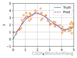
上式是一个非参数的注意力汇聚（nonparametric attention pooling）模型。 接下来基于这个非参数的注意力汇聚模型绘制的预测结果的模型预测线是平滑的，并且比平均汇聚的预测更接近真实。

# X_repeat的形状:(n_test,n_train),
# 每一行都包含着相同的测试输入（例如：同样的查询）
X_repeat = x_test.repeat_interleave(n_train).reshape((-1, n_train))
# x_train包含着键。attention_weights的形状：(n_test,n_train),
# 每一行都包含着要在给定的每个查询的值（y_train）之间分配的注意力权重
attention_weights = nn.functional.softmax(-(X_repeat - x_train)**2 / 2, dim=1)
# y_hat的每个元素都是值的加权平均值，其中的权重是注意力权重
y_hat = torch.matmul(attention_weights, y_train)
plot_kernel_reg(y_hat)

​

​

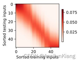
观察注意力的权重可以发现，“查询-键”对越接近，注意力汇聚的注意力权重就越高。

d2l.show_heatmaps(attention_weights.unsqueeze(0).unsqueeze(0),
                  xlabel='Sorted training inputs',
                  ylabel='Sorted testing inputs')

​

​

10.2.4 带参数的注意力汇聚

可以轻松地将可学习的参数集成到注意力汇聚中，例如，在下面的查询 $x$ 和键 $x_i$ 之间的距离乘以可学习参数 $w$：

$$\begin{array}{rl}f(x)=& \sum _{i=1}^n\alpha (x,x_i)y_i\\ =& \sum _{i=1}^n\frac{\exp (-\frac{1}{2}((x-x_i)w{)}^2)}{{\sum }_{j=1}^n\exp (-\frac{1}{2}((x-x_j)w{)}^2)}{y}_i\\ =& \sum _{i=1}^n\mathrm{softmax}\left(-\frac{1}{2}((x-x_i)w{)}^2\right)y_i\end{array}$$

10.2.4.1 批量矩阵乘法

假定两个张量的形状分别是 $(n,a,b)$ 和 $(n,b,c)$，它们的批量矩阵乘法输出的形状为 $(n,a,c)$。
。

X = torch.ones((2, 1, 4))
Y = torch.ones((2, 4, 6))
torch.bmm(X, Y).shape

torch.Size([2, 1, 6])

可以使用小批量矩阵乘法来计算小批量数据中的加权平均值。

weights = torch.ones((2, 10)) * 0.1
values = torch.arange(20.0).reshape((2, 10))
weights.shape, values.shape, weights.unsqueeze(1).shape, values.unsqueeze(-1).shape, torch.bmm(weights.unsqueeze(1), values.unsqueeze(-1))

(torch.Size([2, 10]),
 torch.Size([2, 10]),
 torch.Size([2, 1, 10]),
 torch.Size([2, 10, 1]),
 tensor([[[ 4.5000]],
 
         [[14.5000]]]))

10.2.4.2 定义模型

class NWKernelRegression(nn.Module):
    def __init__(self, **kwargs):
        super().__init__(**kwargs)
        self.w = nn.Parameter(torch.rand((1,), requires_grad=True))

    def forward(self, queries, keys, values):
        # queries和attention_weights的形状为(查询个数，“键－值”对个数)
        queries = queries.repeat_interleave(keys.shape[1]).reshape((-1, keys.shape[1]))
        self.attention_weights = nn.functional.softmax(
            -((queries - keys) * self.w)**2 / 2, dim=1)
        # values的形状为(查询个数，“键－值”对个数)
        return torch.bmm(self.attention_weights.unsqueeze(1),
                         values.unsqueeze(-1)).reshape(-1)

10.2.4.3 训练

# X_tile的形状:(n_train，n_train)，每一行都包含着相同的训练输入
X_tile = x_train.repeat((n_train, 1))
# Y_tile的形状:(n_train，n_train)，每一行都包含着相同的训练输出
Y_tile = y_train.repeat((n_train, 1))
# keys的形状:('n_train'，'n_train'-1)
keys = X_tile[(1 - torch.eye(n_train)).type(torch.bool)].reshape((n_train, -1))
# values的形状:('n_train'，'n_train'-1)
values = Y_tile[(1 - torch.eye(n_train)).type(torch.bool)].reshape((n_train, -1))

net = NWKernelRegression()
loss = nn.MSELoss(reduction='none')  # 使用平方损失函数
trainer = torch.optim.SGD(net.parameters(), lr=0.5)  # 使用随机梯度下降
animator = d2l.Animator(xlabel='epoch', ylabel='loss', xlim=[1, 5])

for epoch in range(5):
    trainer.zero_grad()
    l = loss(net(x_train, keys, values), y_train)
    l.sum().backward()
    trainer.step()
    print(f'epoch {epoch + 1}, loss {float(l.sum()):.6f}')
    animator.add(epoch + 1, float(l.sum()))

​

​

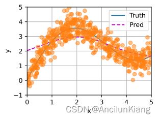
训练完带参数的注意力汇聚模型后可以发现：在尝试拟合带噪声的训练数据时，预测结果绘制的线不如之前非参数模型的平滑。

# keys的形状:(n_test，n_train)，每一行包含着相同的训练输入（例如，相同的键）
keys = x_train.repeat((n_test, 1))
# value的形状:(n_test，n_train)
values = y_train.repeat((n_test, 1))
y_hat = net(x_test, keys, values).unsqueeze(1).detach()
plot_kernel_reg(y_hat)

​

​

与非参数的注意力汇聚模型相比， 带参数的模型加入可学习的参数后， 曲线在注意力权重较大的区域变得更不平滑。

d2l.show_heatmaps(net.attention_weights.unsqueeze(0).unsqueeze(0),
                  xlabel='Sorted training inputs',
                  ylabel='Sorted testing inputs')

​

​

练习

（1）增加训练数据的样本数量，能否得到更好的非参数的 Nadaraya-Watson 核回归模型？

不能。

n_train_more = 500
x_train_more, _ = torch.sort(torch.rand(n_train_more) * 5)

def f(x):
    return 2 * torch.sin(x) + x**0.8

y_train_more = f(x_train_more) + torch.normal(0.0, 0.5, (n_train_more,))
x_test_more = torch.arange(0, 5, 0.01)
y_truth_more = f(x_test_more)

def plot_kernel_regv_more(y_hat_more):
    d2l.plot(x_test_more, [y_truth_more, y_hat_more], 'x', 'y', legend=['Truth', 'Pred'],
             xlim=[0, 5], ylim=[-1, 5])
    d2l.plt.plot(x_train_more, y_train_more, 'o', alpha=0.5);

X_repeat_more = x_test_more.repeat_interleave(n_train_more).reshape((-1, n_train_more))
attention_weights_more = nn.functional.softmax(-(X_repeat_more - x_train_more)**2 / 2, dim=1)
y_hat_more = torch.matmul(attention_weights_more, y_train_more)
plot_kernel_regv_more(y_hat_more)

​

​

d2l.show_heatmaps(attention_weights_more.unsqueeze(0).unsqueeze(0),
                  xlabel='Sorted training inputs',
                  ylabel='Sorted testing inputs')

​

​

---

（2）在带参数的注意力汇聚的实验中学习得到的参数 $w$ 的价值是什么？为什么在可视化注意力权重时，它会使加权区域更加尖锐？

$w$ 的价值在于放大注意力，也就是利用 softmax 函数的特性使键 $x_i$ 和查询 $x$ 距离小的得以保存，学习到的 $w$ 就是掌握这个放大的尺度。

距离大的被过滤，当然也就显得更尖锐了。

---

（3）如何将超参数添加到非参数的Nadaraya-Watson核回归中以实现更好地预测结果？

加进去就能行。

n_train_test = 50
x_train_test, _ = torch.sort(torch.rand(n_train_test) * 5)

def f(x):
    return 2 * torch.sin(x) + x**0.8

y_train_test = f(x_train_test) + torch.normal(0.0, 0.5, (n_train_test,))
x_test_test = torch.arange(0, 5, 0.1)
y_truth_test = f(x_test_test)

def plot_kernel_regv_more(y_hat_test):
    d2l.plot(x_test_test, [y_truth_test, y_hat_test], 'x', 'y', legend=['Truth', 'Pred'],
             xlim=[0, 5], ylim=[-1, 5])
    d2l.plt.plot(x_train_test, y_train_test, 'o', alpha=0.5);

X_repeat_test = x_test_test.repeat_interleave(n_train_test).reshape((-1, n_train_test))
attention_weights_test = nn.functional.softmax(-((X_repeat_test - x_train_test)*net.w.detach().numpy())**2 / 2, dim=1)  # 加入训练好的权重
y_hat_test = torch.matmul(attention_weights_test, y_train_test)
plot_kernel_regv_more(y_hat_test)

​

​

---

（4）为本节的核回归设计一个新的带参数的注意力汇聚模型。训练这个新模型并可视化其注意力权重。

不会，略。