【随机过程】布朗运动
这里写目录标题
- Brownian motion
Brownian motion
The brownian motion 1D and brownian motion 2D functions, written with the cumsum command and without for loops, are used to generate a one-dimensional and two-dimensional Brownian motion, respectively.
使用cumsum命令编写的布朗运动1D函数和不带for循环的布朗运动2D函数分别生成一维和二维布朗运动。
These Wiener processes are characterized by normal-centered increments with variance h, where h is the time increment, generated by the command randn(1,n)*sqrt(h).
这些维纳过程的特征是方差为h的正态中心增量,其中h是时间增量,由命令randn(1,n)*sqrt(h)生成。
We consider a time interval T = 1000, divided into n = 1000 increments of value h = 1.
我们考虑一个时间间隔T = 1000,分成n = 1000个值h = 1的增量。
Figure1 shows, for example, two trajectories W(t) of a one-dimensional Wiener process.
例如,图1显示了一维维纳过程的两条轨迹W(t)。
 Figure 1 { Two examples of trajectories as a function of the time t of a Wiener process W(t) in one
dimension.
图1{两个关于一维维纳过程W(t)时间t的轨迹函数的例子。
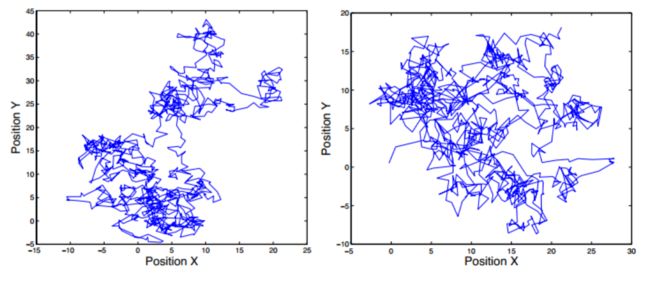
Figure 2,on the other hand, shows two examples of a two-dimensional Brownian motion trajectory, this time as a function of the X and Y spatial coordinates.
另一方面,图2显示了两个二维布朗运动轨迹的例子,这一次是X和Y空间坐标的函数。

Figure 2 -Two examples of trajectories of a two dimensional Wiener process in the plane XY .
图2-在XY平面上二维维纳过程的轨迹的两个例子。
Given N (number of steps), M (number of trajectories) and T (maximum of the time interval),
we generate a matrix W all containing M trajectories of the Brownian motion in one dimension
on the interval [0; T] with a discretization step h = T=N.
给定N(步数),M(轨迹数)和T(时间间隔的最大值),我们生成一个矩阵W,其中包含布朗运动在一维中的M个轨迹,在区间[0;T],离散步长h = T=N。
Figure 3 shows M = 10; 100; 1000 trajectories over the interval [0; 10] with N = 1000 steps.
图3显示M = 10;100;在区间[0;10] N = 1000步。

Figure 3 { M = 10; 100; 1000 (from left to right) trajectories of a one-dimensional Wiener process
over the time interval [0; 10] with N = 1000 discretisation steps.
图3 {M = 10;100;1000个(从左到右)一维维纳过程在时间区间[0;10], N = 1000离散步长。
We simulate M = 1000 trajectories over the interval [0; 10]. Figure 4 shows the mean and
the variance over time of these trajectories.
我们在区间[0;10]。图4显示了这些轨迹随时间的平均值和方差。

Figure 4 { Mean and variance of M = 1000 trajectories of a Brownian motion in one dimension.
图4 {M = 1000条布朗运动轨迹在一维中的均值和方差。
In contrast, figure 5 shows the expectation valuesE[W(t)], E[W(t)2] et E[W(t)4] obtained numerically as a function of time.
与此相反,图5给出了期望值E[W(t)]、E[W(t) 2]和E[W(t) 4]作为时间函数的数值计算结果。
The first moment corresponds exactly to the average.
第一个力矩正好对应于平均值。
In the presence of a zero mean, the variance is equivalent to the moment E[W(t)2].
在均值为零的情况下,方差等于矩E[W(t) 2]。
The red lines in each panel of Figure 5 show that the equalities E[W(t)] = 0, E[W(t)2] = t, and E[W(t)4] = 3t2 are satisfied.
图5中每个面板中的红线表示满足等式E[W(t)] = 0、E[W(t) 2] = t和E[W(t) 4] = 3t 2。
 Figure 5 { Expectation values E[W(t)], E[W(t)2] and E[W(t)4] calculated numerically and compared with the curves (in red) expected theoretically.
图5{数值计算的期望值E[W(t)]、E[W(t) 2]、E[W(t) 4]与理论期望曲线(红色)对比。