- 2024年Python最全人脸检测实战高级:使用 OpenCV、Python 和 dlib 完成眨眼检测
2401_84691757
程序员pythonopencv开发语言
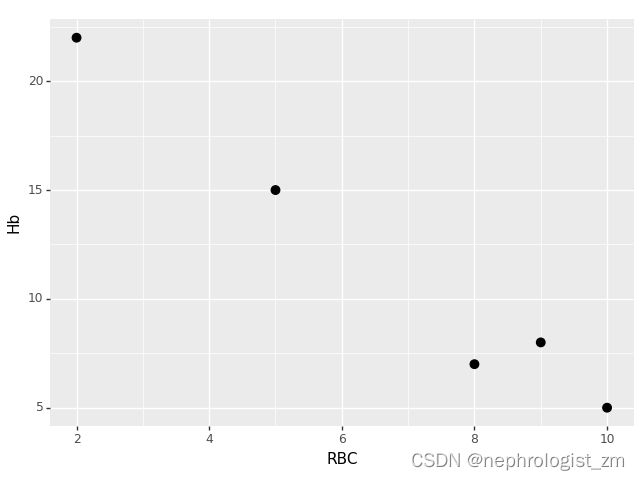
然而,一旦人眨眼(右上),眼睛的纵横比就会急剧下降,接近于零。下图绘制了视频剪辑的眼睛纵横比随时间变化的图表。正如我们所看到的,眼睛纵横比是恒定的,然后迅速下降到接近零,然后再次增加,表明发生了一次眨眼。在下一节中,我们将学习如何使用面部标志、OpenCV、Python和dlib实现眨眼检测的眼睛纵横比。使用面部标志和OpenCV检测眨眼==============================
- Python的内存管理
星辰灬
Pythonpythonpycharm
Python的内存管理在Python中,内存管理涉及到一个包含所有Python对象和数据结构的私有堆(heap)。这个私有堆的管理由内部的Python内存管理器(Pythonmemorymanager)保证。Python内存管理器有不同的组件来处理各种动态存储管理方面的问题,如共享、分割、预分配或缓存。内存管理机制动态内存分配:Python使用动态内存分配,这意味着它在运行时动态分配和管理内存,而
- 【Tkinter从入门到精通】Python原生GUI开发全指南
满怀1015
python开发语言TkinterGUI开发桌面应用界面设计
目录前言️技术背景与价值当前技术痛点️解决方案概述目标读者说明一、技术原理剖析核心概念图解核心作用讲解关键技术模块说明⚖️技术选型对比️二、实战演示⚙️环境配置要求核心代码实现案例1:基础窗口创建案例2:网格布局计算器案例3:文件选择对话框✅运行结果验证⚡三、性能对比测试方法论量化数据对比结果分析四、最佳实践✅推荐方案❌常见错误调试技巧五、应用场景扩展适用领域创新应用方向生态工具链✨结语⚠️技术局
- 【模型部署】如何在Linux中通过脚本文件部署模型
满怀1015
人工智能linux网络人工只能模型部署
在Linux中,你可以将部署命令保存为可执行脚本文件,并通过终端直接调用。以下是几种常见且实用的方法:方法1:Shell脚本(推荐)步骤创建一个.sh文件(例如start_vllm.sh):#!/bin/bashCUDA_VISIBLE_DEVICES=7\python-mvllm.entrypoints.openai.api_server\--served-model-nameQwen2-7B-
- 如果用于AI评课系统的话——五款智能体比较
东方-教育技术博主
人工智能应用人工智能
你目前的项目特点是:已经具备了课堂文本分析、大模型对话系统、课堂视频分析的技术模块;计划通过智能体调用你现有的Python分析脚本,实现数据分析、自动可视化,并与教师互动;更强调多智能体协作、流程灵活编排,以及循证研究的交互分析。因此,我们重点考量生态成熟度、流程编排能力、多智能体协作能力、易用性四个维度。下面逐个分析你提到的框架:智能体框架综合对比分析:框架生态成熟度多智能体能力流程编排能力易用
- 如何用Python实现基础的文生视频AI模型
AI学长带你学AI
AI人工智能与大数据应用开发AI应用开发高级指南python音视频人工智能ai
如何用Python实现基础的文生视频AI模型关键词:文生视频、AI生成、扩散模型、多模态对齐、视频生成算法、Python实现、时间一致性摘要:本文系统讲解基于扩散模型的文生视频(Text-to-Video,T2V)AI模型的核心原理与Python实现方法。从技术背景到数学模型,从算法设计到项目实战,逐步拆解文本-视频跨模态对齐、时间序列建模、扩散生成等关键技术。通过PyTorch实现一个基础版文生
- 【Python GUI框架全解析】六大主流工具对比与实战指南
满怀1015
python开发语言GUI开发PyQtwxPythonKivy
目录前言️技术背景与价值当前技术痛点️解决方案概述目标读者说明一、技术原理剖析核心框架对比图框架定位分析关键技术指标️二、实战演示⚙️环境配置核心代码实现案例1:PyQt5现代化窗口案例2:wxPython文件管理器案例3:Kivy移动风格界面案例4:DearPyGui实时仪表盘✅运行结果验证⚡三、性能对比测试方法论量化数据对比结果分析四、最佳实践✅框架选型建议❌常见误区️调试技巧五、应用场景扩展
- WSL快速在Ubuntu或者Debian安装golang、python、deno、nodejs、java前后端全栈一体化开发环境配置
怪我冷i
云原生ubuntudebiangolangAI写作AI编程
安装golang#移除旧版本(如有)sudoaptremove--autoremove-ygolang#下载最新版(替换为官网最新版本号)wgethttps://go.dev/dl/go1.24.4.linux-amd64.tar.gz#解压到/usr/localsudorm-rf/usr/local/gosudotar-C/usr/local-xzfgo1.24.4.linux-amd64.ta
- python基础知识(二)
目录1.list和tuple1.1.list1.2.tuple2.dict和set2.1.dict2.2.set3.条件3.1.if3.2.if...else3.3.语法糖4.循环4.1.for...in4.2.while1.list和tuple1.1.listPython内置的一种数据类型是列表:list。list是一种有序的集合,可以添加和删除其中的元素。例如:>>>names=['liyan
- Python基础知识(IO编程)
yuxxto56
pythonpython
目录1.文件读写1.1.读文件1.2.字符编码1.3.二进制文件1.4.写文件2.操作文件和目录2.1.环境变量2.2.操作文件、目录1.文件读写读写文件是Python语言最常见的IO操作。通过数据盘读写文件的功能都是由操作系统提供的,读写文件就是请求操作系统打开一个文件对象(通常称为文件描述符),然后,通过操作系统提供的接口从这个文件对象中读取数据(读文件),或者把数据写入这个文件对象(写文件)
- python键盘输入转换为列表_Python键盘输入转换为列表的实例
云云众生w
python键盘输入转换为列表
Python键盘输入转换为列表的实例发布时间:2020-08-1912:58:38来源:脚本之家阅读:92作者:清泉影月Python输入字符串转列表是为了方便后续处理,这种操作在考试的时候比较多见。1.在Python3.0以后,键盘输入使用input函数eg1.>>>x=input>>>123123在命令行没有任何显示,输入123后直接赋值给x,并打印。eg2.>>>x=input("请输入...
- Python中的语法糖介绍
硅星纯牛码
pythonpython
Python中的语法糖介绍1.魔法方法(magicmethods)基础魔法方法属性相关的魔法方法2.装饰器(decorators)内置装饰器@property:让方法变为虚拟属性@classmenthod:定义类方法@staticmethod:定义静态方法functools中的装饰器functoolswraps:保留元数据functoolslru_cache:缓存计算结果3.推导式(compreh
- Python 爬虫实战:12306 订单记录爬取(登录态保持 + 订单数据可视化)
西攻城狮北
python爬虫信息可视化
引言在大数据驱动的今天,12306作为国内最重要的铁路出行平台,积累了海量的出行数据。对于广大用户而言,能够方便地查看和分析自己的出行订单记录,不仅有助于行程管理,还能为未来的出行规划提供有力参考。本文将详细讲解如何利用Python爬虫技术实现12306的模拟登录,爬取个人订单记录,并通过数据可视化技术直观展示出行情况。一、环境搭建与准备工作(一)Python环境配置确保本地已安装Python3.
- 2.setuptools使用
行循自然-kimi
深度学习python
setuptools使用安装pippipinstallsetuptoolsapt源安装apt-getinstallpython-setuptools使用模块安装easy_installpackage-name模块卸载easy_install-mpackage-name使用setuptools来配置工程在工程目录下面新建setup.py.增加内容fromsetuptoolsimportsetup,f
- Python每日一库:setuptools - 现代Python包分发工具
Aerkui
Python库学习python开发语言
1.库简介setuptools是Python生态系统中最重要的包分发工具之一,它是distutils的增强版,提供了更多功能和更好的用户体验。setuptools不仅支持基本的包分发功能,还提供了依赖管理、入口点、开发模式等高级特性,是现代Python包开发的标准工具。2.安装方法pipinstallsetuptools3.核心功能详解3.1创建setup.py文件fromsetuptoolsim
- 探索Gemini Balance:Google Gemini API的代理与负载均衡解决方案
几道之旅
人工智能智能体及数字员工负载均衡运维人工智能
引言在人工智能领域,API的高效使用和管理至关重要。尤其是当涉及到Google的GeminiAPI时,为了实现更稳定、更高效的服务,我们需要一个强大的代理和负载均衡工具。今天,我们就来深入了解一下GeminiBalance这个开源项目,它为GeminiAPI的使用提供了全面而灵活的解决方案。项目概述GeminiBalance是一个基于PythonFastAPI构建的应用程序,主要用于提供Googl
- 提名 Apache ShardingSphere Committer,说说方法
优质资源分享学习路线指引(点击解锁)知识定位人群定位Python实战微信订餐小程序进阶级本课程是pythonflask+微信小程序的完美结合,从项目搭建到腾讯云部署上线,打造一个全栈订餐系统。Python量化交易实战入门级手把手带你打造一个易扩展、更安全、效率更高的量化交易系统文章首发在公众号(龙台的技术笔记),之后同步到博客园和个人网站:xiaomage.info就在前几天,收到了ApacheS
- python内置函数——enumerate()
Believer_abby
python内置函数python
说明:emumerate()函数用于将一个可遍历的序列(如列表,元组或字符串)组合为一个索引序列,同时列出数据和数据下标,一般用在for循环中。语法:enumerate(sequence,[start=0])参数:sequence:表示一个序列、迭代器或其他支持迭代的对象;start:下标起始位置,默认为0。使用:seasons=['spring','summer','fall','winter'
- 【Python基础】07 实战:批量视频压缩的实现
智算菩萨
python服务器开发语言
前言在数字化时代,视频内容已成为信息传播的主要载体。无论是个人用户还是企业,都面临着大量视频文件存储和传输的挑战。视频文件通常体积庞大,占用大量存储空间,同时在网络传输时也会消耗大量带宽。因此,一个高效、易用的视频压缩工具变得尤为重要。本文将详细介绍一个基于Python开发的批量视频压缩工具,该工具结合了现代图形界面设计和强大的FFmpeg视频处理能力,为用户提供了一站式的视频压缩解决方案。通过本
- 男模Python 函数命名以及鸡兔同笼函数
pythonyuanke
python开发语言
那么问你一个问题,现在是不是所有的函数都是def开头的?如果def就是函数的名字,那么python怎么区分该调用哪一个函数?名字都一样啊那也就是def后面的是函数名字?def后面,括号前面参数列表,这里的参数指的是形式参数,就是括号里面的部分这里只有一个形式参数,所以没有逗号,如果有多个形式参数,那么用逗号分隔参考我们在world.py里面写的几个函数,比如defadd(a,b)你说一下它的名字和
- Python 开发规范:pdb & cProfile:调试 & 性能分析
写文章的大米
Python核心技术python
↑↑↑欢迎点赞、关注、收藏!!!,10年IT行业老鸟,持续分享更多IT干货文章目录pdb&cProfile:调试&性能分析核心内容1、调试和性能分析的必要性2、pdb调试工具3、cProfile性能分析工具pdb&cProfile:调试&性能分析核心内容1、调试和性能分析的必要性在实际生产环境中,代码调试(找问题根因、修复bug)和性能分析(优化效率、减少latency)是开发关键环节。尤其,面对
- Python私有属性:隐藏数据的秘密武器
有奇妙能力吗
知识分享Pythonpython开发语言
Python私有属性详解:为什么我们需要“隐藏”对象的数据?一、引言在面向对象编程中,封装(Encapsulation)是三大基本特性之一(另外两个是继承和多态)。而“私有属性”就是实现封装的重要手段之一。在Python中虽然不像Java或C++那样严格区分访问权限,但依然提供了一种机制来限制对类内部属性的直接访问。本文将带你深入了解:什么是私有属性?如何定义私有属性?私有属性的原理与注意事项使用
- Python中filter()函数详解
有奇妙能力吗
Python知识分享python开发语言
什么是filter()?filter()是Python内置的一个函数,它的作用是:从一个可迭代对象(如列表、元组等)中筛选出符合条件的元素,生成一个新的迭代器。你可以把它理解成一个“过滤器”:你给它一堆数据和一个筛选条件,它会帮你把符合这个条件的数据挑出来。基本语法filter(函数,可迭代对象)第一个参数是一个函数,它用来判断每个元素是否符合条件。第二个参数是一个可迭代对象,比如列表、元组、字符
- Python命名空间:名字管理的秘密
什么是命名空间?你可以把命名空间想象成一个“名字的电话簿”:它记录了你程序中使用的各种名字(变量名、函数名、类名等)和它们对应的内容。比如你写了一个变量x=10,Python就会在某个命名空间里记下:“哦,用户用了x这个名字,它代表的是10。”命名空间的类型(就像不同的电话本)Python中有几种不同作用范围的命名空间,我们可以理解为是不同层级的“电话本”:1.内置命名空间(Built-inNam
- python中的运算符
走过..
python开发语言
目录文章目录前言一、算数运算符1.算数运算符包括+,-,*,/,**,//,%1.1、加减乘除(+,-,*,/)运算符的使用1.2、**是求次方m的n次方1.3、%是求余,m%2可以用来验证奇数偶数0为偶,1为奇数。m%n有n中情况,m%n==0证明m是n的倍数。二、赋值运算符1.赋值运算符有=,+=,-=,*=,/=,//=,**=,%=1.1赋予(=)1.2(+,-,*,/,**,//,%)=
- 【Python 中的几类运算符】
文章目录文章目录一、算术运算符二、比较运算符三、赋值运算符四、逻辑运算符附加知识:五、其他运算符1.位运算符2.成员运算符3.身份运算符总结一、算术运算符加法(+):用于两个数值相加。例如,a=5,b=3,a+b的结果为8。也可以用于字符串拼接,如"Hello,"+"World"的结果为"Hello,World"。示例:a=5b=3result=a+bprint("求和",result)a="He
- Windows PowerShell中无法将"python"项识别为cmdlet、函数、脚本文件或可运行程序的名称
xqhrs232
ROS系统/Python
原文地址::https://blog.csdn.net/Blateyang/article/details/86421594相关文章1、如何在Powershell中运行python程序?----https://cloud.tencent.com/developer/ask/1426072、Windows下如何方便的运行py脚本----https://blog.csdn.net/Naisu_kun/
- Vscode中Python无法将pip/pytest”项识别为 cmdlet、函数、脚本文件或可运行程序的名称
在Python需要pip下载插件时报错,是因为没有把Python安装路径下的Scripts添加到系统的path路径中。如果到了对应路径没发现pip文件,查看是否有pip相关文件,一般会存在pip3命令行使用pip3install后会进行提示更新,按照提示进行更新即可bug2:通过piplist发现其实已经安装pytest但使用pytest--version提示相同错误可通过pipuninstall
- Python中if name == ‘main‘的妙用
el psy congroo
Pythonpython
参考:Python中的ifname==‘main’是干嘛的?先运行下面代码:print(__name__)if__name__=="__main__":print(__name__)print("helloworld")print(__name__)当py文件作为主程序直接运行时,__name__无论在哪都是__main__那if__name__=="__main__"有什么用呢?一个py文件也是
- Python爬取与可视化-豆瓣电影数据
木子空间Pro
项目集锦#课程设计python信息可视化开发语言
引言在数据科学的学习过程中,数据获取与数据可视化是两项重要的技能。本文将展示如何通过Python爬取豆瓣电影Top250的电影数据,并将这些数据存储到数据库中,随后进行数据分析和可视化展示。这个项目涵盖了从数据抓取、存储到数据可视化的整个过程,帮助大家理解数据科学项目的全流程。环境配置与准备工作在开始之前,我们需要确保安装了一些必要的库:urllib:用于发送HTTP请求和获取网页数据Beauti
- 对于规范和实现,你会混淆吗?
yangshangchuan
HotSpot
昨晚和朋友聊天,喝了点咖啡,由于我经常喝茶,很长时间没喝咖啡了,所以失眠了,于是起床读JVM规范,读完后在朋友圈发了一条信息:
JVM Run-Time Data Areas:The Java Virtual Machine defines various run-time data areas that are used during execution of a program. So
- android 网络
百合不是茶
网络
android的网络编程和java的一样没什么好分析的都是一些死的照着写就可以了,所以记录下来 方便查找 , 服务器使用的是TomCat
服务器代码; servlet的使用需要在xml中注册
package servlet;
import java.io.IOException;
import java.util.Arr
- [读书笔记]读法拉第传
comsci
读书笔记
1831年的时候,一年可以赚到1000英镑的人..应该很少的...
要成为一个科学家,没有足够的资金支持,很多实验都无法完成
但是当钱赚够了以后....就不能够一直在商业和市场中徘徊......
- 随机数的产生
沐刃青蛟
随机数
c++中阐述随机数的方法有两种:
一是产生假随机数(不管操作多少次,所产生的数都不会改变)
这类随机数是使用了默认的种子值产生的,所以每次都是一样的。
//默认种子
for (int i = 0; i < 5; i++)
{
cout<<
- PHP检测函数所在的文件名
IT独行者
PHP函数
很简单的功能,用到PHP中的反射机制,具体使用的是ReflectionFunction类,可以获取指定函数所在PHP脚本中的具体位置。 创建引用脚本。
代码:
[php]
view plain
copy
// Filename: functions.php
<?php&nbs
- 银行各系统功能简介
文强chu
金融
银行各系统功能简介 业务系统 核心业务系统 业务功能包括:总账管理、卡系统管理、客户信息管理、额度控管、存款、贷款、资金业务、国际结算、支付结算、对外接口等 清分清算系统 以清算日期为准,将账务类交易、非账务类交易的手续费、代理费、网络服务费等相关费用,按费用类型计算应收、应付金额,经过清算人员确认后上送核心系统完成结算的过程 国际结算系
- Python学习1(pip django 安装以及第一个project)
小桔子
pythondjangopip
最近开始学习python,要安装个pip的工具。听说这个工具很强大,安装了它,在安装第三方工具的话so easy!然后也下载了,按照别人给的教程开始安装,奶奶的怎么也安装不上!
第一步:官方下载pip-1.5.6.tar.gz, https://pypi.python.org/pypi/pip easy!
第二部:解压这个压缩文件,会看到一个setup.p
- php 数组
aichenglong
PHP排序数组循环多维数组
1 php中的创建数组
$product = array('tires','oil','spark');//array()实际上是语言结构而不 是函数
2 如果需要创建一个升序的排列的数字保存在一个数组中,可以使用range()函数来自动创建数组
$numbers=range(1,10)//1 2 3 4 5 6 7 8 9 10
$numbers=range(1,10,
- 安装python2.7
AILIKES
python
安装python2.7
1、下载可从 http://www.python.org/进行下载#wget https://www.python.org/ftp/python/2.7.10/Python-2.7.10.tgz
2、复制解压
#mkdir -p /opt/usr/python
#cp /opt/soft/Python-2
- java异常的处理探讨
百合不是茶
JAVA异常
//java异常
/*
1,了解java 中的异常处理机制,有三种操作
a,声明异常
b,抛出异常
c,捕获异常
2,学会使用try-catch-finally来处理异常
3,学会如何声明异常和抛出异常
4,学会创建自己的异常
*/
//2,学会使用try-catch-finally来处理异常
- getElementsByName实例
bijian1013
element
实例1:
<!DOCTYPE html PUBLIC "-//W3C//DTD XHTML 1.0 Transitional//EN" "http://www.w3.org/TR/xhtml1/DTD/xhtml1-transitional.dtd">
<html xmlns="http://www.w3.org/1999/x
- 探索JUnit4扩展:Runner
bijian1013
java单元测试JUnit
参加敏捷培训时,教练提到Junit4的Runner和Rule,于是特上网查一下,发现很多都讲的太理论,或者是举的例子实在是太牵强。多搜索了几下,搜索到两篇我觉得写的非常好的文章。
文章地址:http://www.blogjava.net/jiangshachina/archive/20
- [MongoDB学习笔记二]MongoDB副本集
bit1129
mongodb
1. 副本集的特性
1)一台主服务器(Primary),多台从服务器(Secondary)
2)Primary挂了之后,从服务器自动完成从它们之中选举一台服务器作为主服务器,继续工作,这就解决了单点故障,因此,在这种情况下,MongoDB集群能够继续工作
3)挂了的主服务器恢复到集群中只能以Secondary服务器的角色加入进来
2
- 【Spark八十一】Hive in the spark assembly
bit1129
assembly
Spark SQL supports most commonly used features of HiveQL. However, different HiveQL statements are executed in different manners:
1. DDL statements (e.g. CREATE TABLE, DROP TABLE, etc.)
- Nginx问题定位之监控进程异常退出
ronin47
nginx在运行过程中是否稳定,是否有异常退出过?这里总结几项平时会用到的小技巧。
1. 在error.log中查看是否有signal项,如果有,看看signal是多少。
比如,这是一个异常退出的情况:
$grep signal error.log
2012/12/24 16:39:56 [alert] 13661#0: worker process 13666 exited on s
- No grammar constraints (DTD or XML schema).....两种解决方法
byalias
xml
方法一:常用方法 关闭XML验证
工具栏:windows => preferences => xml => xml files => validation => Indicate when no grammar is specified:选择Ignore即可。
方法二:(个人推荐)
添加 内容如下
<?xml version=
- Netty源码学习-DefaultChannelPipeline
bylijinnan
netty
package com.ljn.channel;
/**
* ChannelPipeline采用的是Intercepting Filter 模式
* 但由于用到两个双向链表和内部类,这个模式看起来不是那么明显,需要仔细查看调用过程才发现
*
* 下面对ChannelPipeline作一个模拟,只模拟关键代码:
*/
public class Pipeline {
- MYSQL数据库常用备份及恢复语句
chicony
mysql
备份MySQL数据库的命令,可以加选不同的参数选项来实现不同格式的要求。
mysqldump -h主机 -u用户名 -p密码 数据库名 > 文件
备份MySQL数据库为带删除表的格式,能够让该备份覆盖已有数据库而不需要手动删除原有数据库。
mysqldump -–add-drop-table -uusername -ppassword databasename > ba
- 小白谈谈云计算--基于Google三大论文
CrazyMizzz
Google云计算GFS
之前在没有接触到云计算之前,只是对云计算有一点点模糊的概念,觉得这是一个很高大上的东西,似乎离我们大一的还很远。后来有机会上了一节云计算的普及课程吧,并且在之前的一周里拜读了谷歌三大论文。不敢说理解,至少囫囵吞枣啃下了一大堆看不明白的理论。现在就简单聊聊我对于云计算的了解。
我先说说GFS
&n
- hadoop 平衡空间设置方法
daizj
hadoopbalancer
在hdfs-site.xml中增加设置balance的带宽,默认只有1M:
<property>
<name>dfs.balance.bandwidthPerSec</name>
<value>10485760</value>
<description&g
- Eclipse程序员要掌握的常用快捷键
dcj3sjt126com
编程
判断一个人的编程水平,就看他用键盘多,还是鼠标多。用键盘一是为了输入代码(当然了,也包括注释),再有就是熟练使用快捷键。 曾有人在豆瓣评
《卓有成效的程序员》:“人有多大懒,才有多大闲”。之前我整理了一个
程序员图书列表,目的也就是通过读书,让程序员变懒。 程序员作为特殊的群体,有的人可以这么懒,懒到事情都交给机器去做,而有的人又可以那么勤奋,每天都孜孜不倦得
- Android学习之路
dcj3sjt126com
Android学习
转自:http://blog.csdn.net/ryantang03/article/details/6901459
以前有J2EE基础,接触JAVA也有两三年的时间了,上手Android并不困难,思维上稍微转变一下就可以很快适应。以前做的都是WEB项目,现今体验移动终端项目,让我越来越觉得移动互联网应用是未来的主宰。
下面说说我学习Android的感受,我学Android首先是看MARS的视
- java 遍历Map的四种方法
eksliang
javaHashMapjava 遍历Map的四种方法
转载请出自出处:
http://eksliang.iteye.com/blog/2059996
package com.ickes;
import java.util.HashMap;
import java.util.Iterator;
import java.util.Map;
import java.util.Map.Entry;
/**
* 遍历Map的四种方式
- 【精典】数据库相关相关
gengzg
数据库
package C3P0;
import java.sql.Connection;
import java.sql.SQLException;
import java.beans.PropertyVetoException;
import com.mchange.v2.c3p0.ComboPooledDataSource;
public class DBPool{
- 自动补全
huyana_town
自动补全
<!DOCTYPE html PUBLIC "-//W3C//DTD XHTML 1.0 Transitional//EN" "http://www.w3.org/TR/xhtml1/DTD/xhtml1-transitional.dtd"><html xmlns="http://www.w3.org/1999/xhtml&quo
- jquery在线预览PDF文件,打开PDF文件
天梯梦
jquery
最主要的是使用到了一个jquery的插件jquery.media.js,使用这个插件就很容易实现了。
核心代码
<!DOCTYPE html PUBLIC "-//W3C//DTD XHTML 1.0 Transitional//EN" "http://www.w3.org/TR/xhtml1/DTD/xhtml1-transitional.
- ViewPager刷新单个页面的方法
lovelease
androidviewpagertag刷新
使用ViewPager做滑动切换图片的效果时,如果图片是从网络下载的,那么再子线程中下载完图片时我们会使用handler通知UI线程,然后UI线程就可以调用mViewPager.getAdapter().notifyDataSetChanged()进行页面的刷新,但是viewpager不同于listview,你会发现单纯的调用notifyDataSetChanged()并不能刷新页面
- 利用按位取反(~)从复合枚举值里清除枚举值
草料场
enum
以 C# 中的 System.Drawing.FontStyle 为例。
如果需要同时有多种效果,
如:“粗体”和“下划线”的效果,可以用按位或(|)
FontStyle style = FontStyle.Bold | FontStyle.Underline;
如果需要去除 style 里的某一种效果,
- Linux系统新手学习的11点建议
刘星宇
编程工作linux脚本
随着Linux应用的扩展许多朋友开始接触Linux,根据学习Windwos的经验往往有一些茫然的感觉:不知从何处开始学起。这里介绍学习Linux的一些建议。
一、从基础开始:常常有些朋友在Linux论坛问一些问题,不过,其中大多数的问题都是很基础的。例如:为什么我使用一个命令的时候,系统告诉我找不到该目录,我要如何限制使用者的权限等问题,这些问题其实都不是很难的,只要了解了 Linu
- hibernate dao层应用之HibernateDaoSupport二次封装
wangzhezichuan
DAOHibernate
/**
* <p>方法描述:sql语句查询 返回List<Class> </p>
* <p>方法备注: Class 只能是自定义类 </p>
* @param calzz
* @param sql
* @return
* <p>创建人:王川</p>
* <p>创建时间:Jul