基于模拟退火算法的TSP问题建模求解(Python)
基于模拟退火算法的TSP问题建模求解(Python)
- 一、模拟退火算法(Simulated Annealing Algorithm,SAA)工程背景
-
- 模拟退火算法用于优化问题求解原理
- 二、旅行商问题(Travelling salesman problem,TSP)
-
- TSP问题数学模型
- 三、基于模拟退火算法的TSP问题建模求解
-
- 3.1实例分析
-
- 3.1.1导入库
- 3.1.2数据
- 3.1.3生成初始解
- 3.1.4扰动生成新解
- 3.1.5评价函数
- 3.1.6Metropolis接受准则
- 3.1.7模拟退火算法
- 3.2完整代码
- 3.3求解结果
一、模拟退火算法(Simulated Annealing Algorithm,SAA)工程背景
模拟退火算法(Simulated Annealing Algorithm)来源于固体退火原理,是一种基于概率的算法。将固体加温至充分高的温度,再让其徐徐冷却,加温时,固体内部粒子随温升变为无序状,内能增大,分子和原子越不稳定。而徐徐冷却时粒子渐趋有序,能量减少,原子越稳定。在冷却(降温)过程中,固体在每个温度都达到平衡态,最后在常温时达到基态,内能减为最小。模拟退火算法从某一较高初温出发,伴随温度参数的不断下降,结合概率突跳特性在解空间中随机寻找目标函数的全局最优解,即在局部最优解能概率性地跳出并最终趋于全局最优。模拟退火算法是通过赋予搜索过程一种时变且最终趋于零的概率突跳性,从而可有效避免陷入局部极小并最终趋于全局最优的串行结构的优化算法。
模拟退火算法用于优化问题求解原理
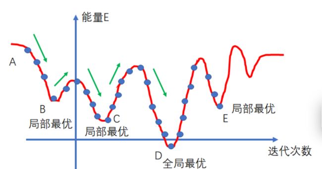
模拟退火算法包含两个部分即Metropolis算法和退火过程,分别对应内循环和外循环。外循环就是退火过程,将固体达到较高的温度(初始温度 T 0 T_0 T0),然后按照降温系数 α \alpha α使温度按照一定的比例下降,当达到终止温度 T f T_f Tf时,冷却结束,即退火过程结束;Metropolis算法是内循环,即在每次温度下,迭代L次,寻找在该温度下能量的最小值(即最优解)。下图中所示即为在一次温度下,跌代L次,固体能量发生的变化。
在该温度下,整个迭代过程中温度不发生变化,能量发生变化,当前一个状态x(n)的能量大于后一个状态x(n+1)的能量时,状态x(n)的解没有状态x(n+1)的解好,所以接受状态x(n+1),以 P = 1 P=1 P=1的概率接受。但是如果下一状态的能量比前一个状态的能量高时,则接受下一状态的概率为 P = e E ( n + 1 ) − E ( n ) T P=\text{e}^{\frac{E(n+1)-E(n)}{T}} P=eTE(n+1)−E(n)
P = { 1 E ( n + 1 ) < E ( n ) e E ( n + 1 ) − E ( n ) T E ( n + 1 ) ≥ E ( n ) P=\begin{cases} 1 & E(n+1) < E(n) \\ \text{e}^{\frac{E(n+1)-E(n)}{T}} & E(n+1) \geq E(n) \\ \end{cases} P={1eTE(n+1)−E(n)E(n+1)<E(n)E(n+1)≥E(n)
- E(n):状态为x(n)时系统的能量,即TSP问题中目标函数值
- T:当前温度,控制退火速率,即温度下降,最简单的下降方式是指数式下降:T(n) = α \alpha α T(n) ,n =1,2,3,…其中 α \alpha α是小于1的正数,一般取值为0.8到0.99之间。使的对每一温度,有足够的转移尝试,指数式下降的收敛速度比较慢。
用固体退火模拟组合优化问题,状态x(n)映射为问题的解,将内能E模拟为目标函数值f,温度T演化成控制迭代过程参数t,即得到解组合优化问题的模拟退火算法:由初始解i和控制参数初值t开始,对当前解重复“产生新解→计算目标函数差→接受或舍弃”的迭代,并逐步衰减t值,算法终止时的当前解即为所得近似最优解,退火过程由冷却进度表(Cooling Schedule)控制,包括控制参数的初值t及其衰减因子Δt、每个t值时的迭代次数L和停止条件Tf。而温度的作用就是来计算转移概率P的。当温度每次下降后,转移概率也发生变化,因此在所有温度下迭代L次的结果也都是不相同的。在每个温度下迭代L次来寻找当前温度下的最优解,然后降低温度继续寻找,直到到达终止温度,即转移概率P接近于0
对应于优化问题(min问题),如果当前解的目标函数值<新解的目标函数值,则无条件接受;如果当前解的目标函数值>=新解的目标函数值,以一定的概率接受新解作为当前解。
Metropolis算法就是如何在局部最优解的情况下让其跳出来(如图中B、C、E为局部最优),是退火的基础。1953年Metropolis提出重要性采样方法,即以概率来接受新状态,而不是使用完全确定的规则,称为Metropolis准则,计算量较低。
假设初始解为A,多次迭代之后更新到B的局部最优解,这时发现更新到解B时,目标函数值比A要低,则说明接近最优解了,因此百分百转移,到达解B后,发现下一步目标函数值上升了,如果是梯度下降则是不允许继续向前的,而这里会以一定的概率跳出这个坑,这各概率和当前的状态、能量等都有关系。在一开始需要T值较大,这样根据函数的单调性,可以看出接受差解的P是较大的,便于对全局进行搜索,而在后期温度下降,T值变小,当温度趋于零时,只能接受目标函数下降的,这有利于尽快收敛,完成迭代。
二、旅行商问题(Travelling salesman problem,TSP)
TSP问题数学模型
刘兴禄 -《运筹优化常用模型、算法及案例实战:Python+Java实现》总结了TSP问题共有3种数学模型:
- Dantzig-Fulkerson-Johnson model,DFJ模型(本文采用)
- Miller-Tucker-Zemlin model,MTZ模型
- 1-tree模型
DFJ模型,也是最常见的模型如下:
min ∑ i ∈ V ∑ j ∈ V d i j x i j subject to ∑ j ∈ V x i j = 1 , ∀ i ∈ V , i ≠ j ∑ i ∈ V x i j = 1 , ∀ j ∈ V , i ≠ j ∑ i , j ∈ S x i j ≤ ∣ S ∣ − 1 , 2 ≤ ∣ S ∣ ≤ N − 1 , S ⊂ V x i j ∈ { 0 , 1 } , ∀ i , j ∈ V \begin{align} \min \quad & \sum_{i \in V}{}\sum_{j \in V} d_{ij}x_{ij}\\ \text{subject to} \quad &\sum_{j \in V} x_{ij} = 1, \quad \forall i \in V,i \neq j \\ &\sum_{i \in V}{x_{ij}} =1,\quad \forall j \in V ,i \neq j\\ & {\sum_{i,j \in S}{x_{ij}} \leq |S|-1,\quad 2\leq |S| \leq N-1, S \subset V}\\ &x_{ij} \in \{0,1\}, \quad \forall i,j \in V \end{align} minsubject toi∈V∑j∈V∑dijxijj∈V∑xij=1,∀i∈V,i=ji∈V∑xij=1,∀j∈V,i=ji,j∈S∑xij≤∣S∣−1,2≤∣S∣≤N−1,S⊂Vxij∈{0,1},∀i,j∈V
三、基于模拟退火算法的TSP问题建模求解
3.1实例分析
3.1.1导入库
import numpy as np
import pandas as pd
import matplotlib.pyplot as plt
3.1.2数据
# 数据:城市以及坐标
city_coordinates = {
        0: (60, 200),
        1: (180, 200),
        2: (80, 180),
        3: (140, 180),
        4: (20, 160),
        5: (100, 160),
        6: (200, 160),
        7: (140, 140),
        8: (40, 120),
        9: (100, 120),
        10: (180, 100),
        11: (60, 80),
        12: (120, 80),
        13: (180, 60),
        14: (20, 40),
        15: (100, 40),
        16: (200, 40),
        17: (20, 20),
        18: (60, 20),
        19: (160, 20),
    }
num_city = len(city_coordinates)
f'城市数量: {num_city}'
'城市数量: 20'
# 距离矩阵
distance_matrix = np.empty(shape=(num_city, num_city), dtype=np.float_)
for i in range(num_city):
    xi, yi = city_coordinates[i]
    for j in range(num_city):
        xj, yj = city_coordinates[j]
        distance_matrix[i][j] = np.sqrt(np.power(xi - xj, 2) + np.power(yi - yj, 2))
3.1.3生成初始解
x = np.random.permutation(num_city)  # 初始解,编码采用常规的整数编码,如果城市数目为N,那么解就可以表达为1~N的随机排列,
x
array([ 4, 16, 17,  7,  5, 18, 15,  3,  0, 10,  8,  9, 14,  1, 12, 13,  6,
       11,  2, 19])
3.1.4扰动生成新解
def two_opt(x: np.ndarray):
    """
    2-opt swap,扰动生成新解
    :param x: 解
    :return: 新解
    """
    x = x.copy()
    r1 = np.random.randint(low=0, high=num_city)
    r2 = np.random.randint(low=0, high=num_city)
    x[r1], x[r2] = x[r2], x[r1]
    return x

x_ = two_opt(x)
x_
array([ 4, 16, 17,  9,  5, 18, 15,  3,  0, 10,  8,  7, 14,  1, 12, 13,  6,
       11,  2, 19])
3.1.5评价函数
def eval_func(x):
    """
    评价函数
    :param x: 解
    :return: 解的目标函数值
    """
    total_distance = 0
    for k in range(num_city - 1):
        total_distance += distance_matrix[x[k]][x[k + 1]]
    total_distance += distance_matrix[x[-1]][x[0]]
    return total_distance

objective_value_x = eval_func(x),  # x的目标函数值
objective_value_x_ = eval_func(x_) # x_的目标函数值
objective_value_x, objective_value_x_
((2666.7841429791642,), 2705.4679394931945)
3.1.6Metropolis接受准则
P = { 1 E ( n + 1 ) < E ( n ) e E ( n + 1 ) − E ( n ) T E ( n + 1 ) ≥ E ( n ) P=\begin{cases} 1 & E(n+1) < E(n) \\ \text{e}^{\frac{E(n+1)-E(n)}{T}} & E(n+1) \geq E(n) \\ \end{cases} P={1eTE(n+1)−E(n)E(n+1)<E(n)E(n+1)≥E(n)
- E(n):状态为x(n)时系统的能量,即TSP问题中目标函数值
- T:当前温度,T控制退火速率,即温度下降,最简单的下降方式是指数式下降:T(n) = α \alpha α T(n) ,n =1,2,3,…其中 α \alpha α是小于1的正数,一般取值为0.8到0.99之间。使的对每一温度,有足够的转移尝试,指数式下降的收敛速度比较慢。
temp_current = 1e6
delta_temp = objective_value_x_ - objective_value_x
if delta_temp > 0:
    # 若新解目标函数值更差,则一定概率接受
    if np.random.uniform(0, 1) < 1. / np.exp(delta_temp / temp_current):
        x = x_
else:
    # TSP为极小化问题,若新解目标函数值更小,则无条件接受新解作为当前解
    x = x_
x
array([ 4, 16, 17,  9,  5, 18, 15,  3,  0, 10,  8,  7, 14,  1, 12, 13,  6,
       11,  2, 19])
3.1.7模拟退火算法
def run_simulated_annealing(temp_initial=1e6, temp_final=.1, alpha=.98):
    """
    :param temp_initial: 初始温度T0
    :param temp_final: 终止温度T0
    :param alpha:降温系数
    :return: 每一代最优解, 及解的目标函数值
    """
    temp_current = temp_initial  # 当前温度

    x = np.random.permutation(num_city)  # 初始解,编码采用常规的整数编码,如果城市数目为N,那么解就可以表达为1~N的随机排列,
    obj_value = eval_func(x)  # 初始解目标函数值

    global_best = x  # 全局最优解
    trace: List[Tuple[np.ndarray, float]] = [(x, obj_value)]  # 记录每一代最优解, 及解的目标函数值
    while temp_current > temp_final:  # 外循环:退火过程
        for i in range(1000):  # 内循环
            obj_value_old = eval_func(x)
            x_ = two_opt(x)
            obj_value_new = eval_func(x_)
            delta_temp = obj_value_new - obj_value_old
            if delta_temp > 0:
                if np.random.uniform(0, 1) < 1. / np.exp(delta_temp / temp_current):
                    x = x_
            else:
                x = x_
                global_best = x
        trace.append((global_best, eval_func(global_best)))
        temp_current *= alpha

    return trace
3.2完整代码
import logging
from typing import Dict, List, Tuple

import numpy as np
import matplotlib.pyplot as plt

logging.getLogger('matplotlib').setLevel(logging.WARNING)
# logging.basicConfig(level=logging.DEBUG)
logger = logging.getLogger()
logger.setLevel(logging.DEBUG)


def read_dataset(data=1):
    city_coordinates_ = {
        0: (60, 200),
        1: (180, 200),
        2: (80, 180),
        3: (140, 180),
        4: (20, 160),
        5: (100, 160),
        6: (200, 160),
        7: (140, 140),
        8: (40, 120),
        9: (100, 120),
        10: (180, 100),
        11: (60, 80),
        12: (120, 80),
        13: (180, 60),
        14: (20, 40),
        15: (100, 40),
        16: (200, 40),
        17: (20, 20),
        18: (60, 20),
        19: (160, 20),
    }  # 数据1:城市以及坐标
    city_coordinates_att48 = {
        0: (6734, 1453),
        1: (2233, 10),
        2: (5530, 1424),
        3: (401, 841),
        4: (3082, 1644),
        5: (7608, 4458),
        6: (7573, 3716),
        7: (7265, 1268),
        8: (6898, 1885),
        9: (1112, 2049),
        10: (5468, 2606),
        11: (5989, 2873),
        12: (4706, 2674),
        13: (4612, 2035),
        14: (6347, 2683),
        15: (6107, 669),
        16: (7611, 5184),
        17: (7462, 3590),
        18: (7732, 4723),
        19: (5900, 3561),
        20: (4483, 3369),
        21: (6101, 1110),
        22: (5199, 2182),
        23: (1633, 2809),
        24: (4307, 2322),
        25: (675, 1006),
        26: (7555, 4819),
        27: (7541, 3981),
        28: (3177, 756),
        29: (7352, 4506),
        30: (7545, 2801),
        31: (3245, 3305),
        32: (6426, 3173),
        33: (4608, 1198),
        34: (23, 2216),
        35: (7248, 3779),
        36: (7762, 4595),
        37: (7392, 2244),
        38: (3484, 2829),
        39: (6271, 2135),
        40: (4985, 140),
        41: (1916, 1569),
        42: (7280, 4899),
        43: (7509, 3239),
        44: (10, 2676),
        45: (6807, 2993),
        46: (5185, 3258),
        47: (3023, 1942),
    }  # 数据2:att48.txt 城市以及坐标 答案有4种可能,不向上取整,除根号10是10601;不向上取整,不除根号10是33523;向上取整,除根号10是10628;向上取整,不除根号10是33609
    return city_coordinates_att48 if data == 1 else city_coordinates_


def get_distance_matrix(city_coordinates: Dict[int, Tuple[int, int]]) -> np.ndarray:
    distance_matrix = np.empty(shape=(num_city, num_city), dtype=np.float_)
    for i in range(num_city):
        xi, yi = city_coordinates[i]
        for j in range(num_city):
            xj, yj = city_coordinates[j]
            distance_matrix[i][j] = np.sqrt(np.power(xi - xj, 2) + np.power(yi - yj, 2))
    return distance_matrix


def eval_func(x):
    """
    评价函数
    :param x: 解
    :return: 解的目标函数值
    """
    total_distance = 0
    for k in range(num_city - 1):
        total_distance += distance_matrix[x[k]][x[k + 1]]
    total_distance += distance_matrix[x[-1]][x[0]]
    return total_distance


def two_opt(x: np.ndarray):
    """
    2-opt swap,扰动生成新解
    :param x: 解
    :return: 新解
    """
    x = x.copy()
    r1 = np.random.randint(low=0, high=num_city)
    r2 = np.random.randint(low=0, high=num_city)
    x[r1], x[r2] = x[r2], x[r1]
    return x


def run_simulated_annealing(temp_initial=1e6, temp_final=.1, alpha=.98) -> List:
    """
    :param temp_initial: 初始温度T0
    :param temp_final: 终止温度T0
    :param alpha:降温系数
    :return: 每一代最优解, 及解的目标函数值
    """
    temp_current = temp_initial  # 当前温度

    x = np.random.permutation(num_city)  # 初始解,编码采用常规的整数编码,如果城市数目为N,那么解就可以表达为1~N的随机排列,
    obj_value = eval_func(x)  # 初始解目标函数值

    global_best = x  # 全局最优解
    trace: List[Tuple[np.ndarray, float]] = [(x, obj_value)]  # 记录每一代最优解, 及解的目标函数值
    while temp_current > temp_final:  # 外循环:退火过程
        for i in range(1000):  # 内循环
            obj_value_old = eval_func(x)
            x_ = two_opt(x)
            obj_value_new = eval_func(x_)
            delta_temp = obj_value_new - obj_value_old
            if delta_temp > 0:
                if np.random.uniform(0, 1) < 1. / np.exp(delta_temp / temp_current):
                    x = x_
            else:
                x = x_
                global_best = x
        trace.append((global_best, eval_func(global_best)))
        temp_current *= alpha

    return trace


def draw(trace: List) -> None:
    iteration = np.arange(len(trace))
    obj_value = [trace[i][1] for i in range(len(trace))]
    plt.plot(iteration, obj_value)
    plt.show()
    final_solution, final_obj_value = trace[-1]
    x = []
    y = []
    for city in final_solution:
        city_x, city_y = city_coordinates[city]
        x.append(city_x)
        y.append(city_y)
    city_x, city_y = city_coordinates[final_solution[0]]
    x.append(city_x)
    y.append(city_y)
    plt.plot(x, y, 'o-', alpha=1, linewidth=2)
    plt.show()


def print_solution(trace: List[Tuple[int, int]]) -> None:
    logging.info(f'城市数量: {num_city}')
    initial_solution, initial_obj_value = trace[0]
    final_solution, final_obj_value = trace[-1]
    logging.info(f'initial solution: {initial_solution}, objective value: {initial_obj_value}')
    logging.info(f'final solution: {final_solution}, objective value: {final_obj_value}')


if __name__ == "__main__":
    city_coordinates = read_dataset()
    num_city = len(city_coordinates)
    distance_matrix: np.ndarray = get_distance_matrix(city_coordinates)
    trace = run_simulated_annealing()
    print_solution(trace)
    draw(trace)
3.3求解结果
程序中有两个算例:
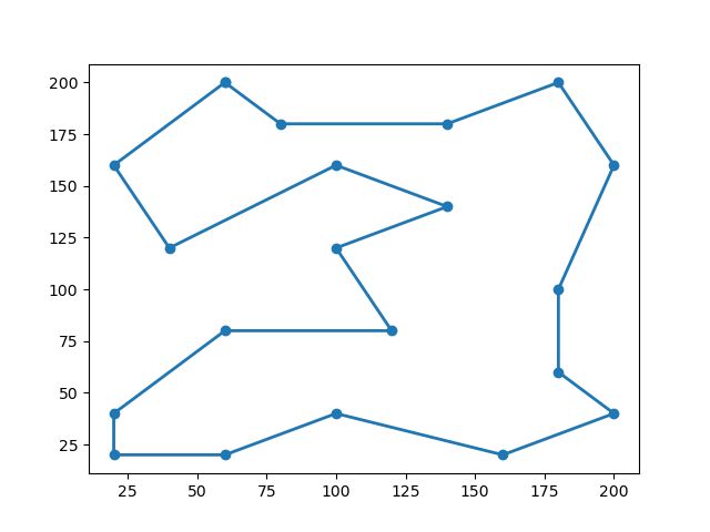
1、 city_coordinates_ ,城市数量为20,本文求解结果目标函数值为911.117353844847;其他文章基于禁忌搜索的TSP问题建模求解(Java)结果为886;基于自适应遗传算法的TSP问题建模求解(Java)为879.0。本文求解结果如下(左图):
INFO:root:城市数量: 20
INFO:root:initial solution: [16  2  9 15  7  3 17 14 19  8 11 12  5  0  4  1 13 10  6 18], objective value: 2040.8676784971715
INFO:root:final solution: [ 1  6 10 13 16 19 12  9 15 18 17 14 11  8  4  0  2  5  7  3], objective value: 911.117353844847
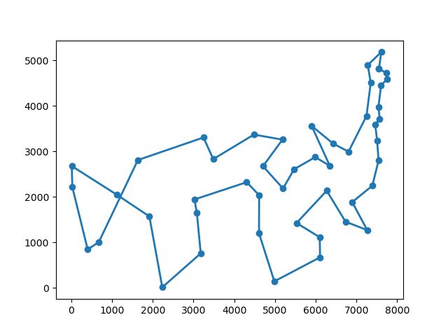
2、 city_coordinates_ att48(TSP问题标准测试函数,城市数量48,最优解为33523)本文求解结果为34974.67245297696(右图):
INFO:root:城市数量: 48
INFO:root:initial solution: [15 22 12 34 24 16 26  3 14  2 27 11 10  0 39  5  4 42 19 44 47 18 28 41  31 36 35 20 43 45 30 46  7 13 33 29  1 23 32 40 38  8 21  9  6 25 37 17], objective value: 162186.17660670803
INFO:root:final solution: [26 18 36  5 27  6 17 43 30 37  8  7  0 39  2 21 15 40 33 13 24 47  4 28 1 41  9 44 34  3 25 23 31 38 20 46 12 22 10 11 14 19 32 45 35 29 42 16], objective value: 34974.67245297696