【强化学习】DQN及其变体网络的原理讲解和代码实现

DQN网络及其变体的实现

一、DQN网络原理回顾

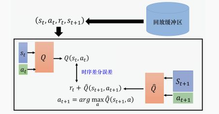
DQN采用经验回放和固定的Q-targets

根据**$ϵ-greedy$**执行行为$a_t$

将经验以$(s_t,a_t,r_{t+1},s_{t+1})$的形式存储到replay memory D

将D中随机抽样一个mini-batch的经验$(s,a,r,s^{\prime })$

用旧的、固定的参数$w^{-}$计算Q-learning target，每隔固定轮数才更新$w^{-}$

在Q-network和Q-learning targets之间优化MSE
$${\mathcal{L}}_i\left(w_i\right)={\mathbb{E}}_{s,a,r,s^{\prime }\sim {\mathcal{D}}_i}\left[{\left(r+\gamma \underset{a^{\prime }}{\max }Q\left(s^{\prime },a^{\prime };w_i^{-}\right)-Q\left(s,a;w_i\right)\right)}^2\right]$$
使用随机梯度下降的方式更新参数

二、DQN代码实现

定义模型

DQN将原来的Q表，也就是每个状态下的每个动作具有一个价值，这样一个二维表改用神经网络来进行代替，这里使用一个多层感知机MLP来实现，输入维度是状态数，输出维度是动作数。

import torch.nn as nn
import torch.nn.functional as F
class MLP(nn.Module):
    def __init__(self, n_states, n_actions, hidden_dim=128):
        super(MLP, self).__init__()
        self.fc1 = nn.Linear(n_states, hidden_dim) #输入层
        self.fc2 = nn.Linear(hidden_dim, hidden_dim) #隐藏层
        self.fc3 = nn.Linear(hidden_dim, n_actions) #输出层
        
    def forward(self, x):
        x = F.relu(self.fc1(x))
        x = F.relu(self.fc2(x))
        return self.fc3(x)

定义经验回放

DQN网络中使用了经验回放，这一方面可以提升样本使用效率，每个样本不会只使用一次后就被丢掉，另一方面是可以减少样本之间的相关性，打乱样本再学习有助于提升训练的稳定性。

具体实现时有两个点，一是要向buffer中添加样本，如果buffer满了就将最早进入的删除，这可以用队列来实现；二是要进行采样，采样的量取决于采样batch的大小。

from collections import deque
import random
class ReplayBuffer(object):
    def __init__(self, capacity: int) -> None:
        self.capacity = capacity
        self.buffer = deque(maxlen = self.capacity)
    
    def sample(self, batch_size: int, sequential: bool = False):
        if(batch_size > len(self.buffer)): #如果批量大小大于经验回放容量大小，则让batch_size大小变为经验回放容量大小
            batch_size = len(self.buffer)
        if sequential: #顺序采样
            rand = random.randint(0, len(self.buffer) - batch_size)
            batch = [self.buffer[i] for i in range(rand, rand + batch_size)]
            return zip(*batch) #将batch中的元组按照列的方式重新组织
            #这里的*运算符是拆包运算符，它会将batch中的元素拆分出来。当我们将这个拆分出来的元素传给zip()函数时，zip()函数会将这些元素按照其相对应的索引位置进行配对，形成一个新的可迭代对象。
            '''
            batch = [(1, 'a', 'A'), (2, 'b', 'B'), (3, 'c', 'C')]
 			zipped = zip(*batch)
			print(list(zipped))
			
			output: [(1, 2, 3), ('a', 'b', 'c'), ('A', 'B', 'C')]
            
            '''
        else: #随机采样
            batch = random.sample(self.buffer, batch_size)
            return zip(*batch)
    
    def clear(self):
        self.buffer.clear()
        
    def __len__(self):
        return len(self.buffer)
    

算法定义

算法定义中比较关键的是更新过程，需要根据损失函数进行梯度下降来更新参数

损失函数定义如下：
$${\mathcal{L}}_i\left(w_i\right)={\mathbb{E}}_{s,a,r,s^{\prime }\sim {\mathcal{D}}_i}\left[{\left(y_i-Q\left(s,a;w_i\right)\right)}^2\right]$$
其中$y_i$计算根据是否为终止状态是不同的
$$y_i=\{\begin{array}{ll}{r}_i& \text{ 对于终止状态 }{s}_{i+1}\\ r_i+\gamma {\max }_{a^{\prime }}Q\left(s_{i+1},a^{\prime };w^{-}\right)& \text{ 对于非终止状态 }{s}_{i+1}\end{array}$$

import torch
import torch.optim as optim
import math
import numpy as np
class DQN:
    def __init__(self, model, memory, cfg):
        self.n_actions = cfg['n_actions']
        self.device = torch.device(cfg['device'])
        self.gamma = cfg['gamma'] #奖励的折扣因子
        
        #关于epsilon-greedy探索策略的相关参数
        self.sample_count = 0  # 用于epsilon的衰减计数
        self.epsilon = cfg['epsilon_start']
        self.sample_count = 0  
        self.epsilon_start = cfg['epsilon_start']
        self.epsilon_end = cfg['epsilon_end']
        self.epsilon_decay = cfg['epsilon_decay']
        self.batch_size = cfg['batch_size']
        
        self.policy_net = model.to(self.device)
        self.target_net = model.to(self.device)
        
        #复制policy_net的参数到target_net，具体训练时target_net的参数是每隔固定轮次从policy_net获得的
        for target_param, param in zip(self.target_net.parameters(), self.policy_net.parameters()): #parameters()返回PyTorch中的可学习参数，例如神经网络层的权重和偏差。
            #使用zip()函数将目标网络和策略网络的对应参数进行配对。这样，我们可以同时遍历两个神经网络的参数。
            #使用data.copy_()方法将策略网络的参数值复制到目标网络的参数中。这里使用copy_()方法是因为我们想要复制参数的值，而不是共享参数的内存地址。
            target_param.data.copy_(param.data)
            
        self.optimizer = optim.Adam(self.policy_net.parameters(), lr=cfg['lr']) #定义优化器
        self.memory = memory #经验回放
        
    def sample_action(self, state):
        self.sample_count += 1
        #epsilon指数衰减
        self.epsilon = self.epsilon_end + (self.epsilon_start = self.epsilon_end) * math.exp(-1 * self.sample_count / self.epsilon_decay)
        if random.random() > self.epsilon:
            with torch.no_grad():
                state = torch.tensor(state, device = self.device, dtype = torch.float32).unsqueeze(dim=0)
                q_values = self.policy_net(state) #将状态state输入到self.policy_net（一个神经网络）中进行前向计算，得到每个动作对应的Q值。
                action = q_values.max(1)[1].item()
                #从Q值中选择具有最大Q值的动作作为最优动作。.max(1)返回Q值中的最大值和对应的索引，
                # [1]表示取索引部分，.item()将索引转换为普通的Python数值，以便进行后续操作。
        else:
                action = random.randrange(self.n_actions)
        return action
    
    @torch.no_grad() # 不计算梯度，该装饰器效果等同于with torch.no_grad()：
    def predict_action(self, state):
        ''' 预测动作
        '''
        state = torch.tensor(state, device=self.device, dtype=torch.float32).unsqueeze(dim=0)
        q_values = self.policy_net(state)
        action = q_values.max(1)[1].item() # 选择Q值最大的动作
        return action
    
    def update(self):
        if len(self.memory) < self.batch_size:
            return
        # 从经验回放中随机采样一个批量的样本
        state_batch, action_batch, reward_batch, next_state_batch, done_batch = self.memory.sample(self.batch_size)
        # 将数据转换为tensor
        state_batch = torch.tensor(np.array(state_batch), device=self.device, dtype=torch.float)
        action_batch = torch.tensor(action_batch, device=self.device).unsqueeze(1)  
        reward_batch = torch.tensor(reward_batch, device=self.device, dtype=torch.float)  
        next_state_batch = torch.tensor(np.array(next_state_batch), device=self.device, dtype=torch.float)
        done_batch = torch.tensor(np.float32(done_batch), device=self.device)
        q_values = self.policy_net(state_batch).gather(dim=1, index=action_batch) # 计算当前状态(s_t,a)对应的Q(s_t, a)
        next_q_values = self.target_net(next_state_batch).max(1)[0].detach() # 计算下一时刻的状态(s_t_,a)对应的Q值
        # 计算期望的Q值，对于终止状态，此时done_batch[0]=1, 对应的expected_q_value等于reward
        expected_q_values = reward_batch + self.gamma * next_q_values * (1-done_batch)
        #当done_batch为1时，表示对应样本是终止状态，此时(1-done_batch)的值为0，表示不考虑未来奖励。
        #因此，对于终止状态，目标Q值只由当前时刻的奖励决定。这种处理方式可以确保在训练过程中，终止状态的目标Q值是正确的，并且不会受到未来状态的影响。
        #这样可以提高训练的稳定性和效果。
        loss = nn.MSELoss()(q_values, expected_q_values.unsqueeze(1))  # 计算均方根损失
        # 优化更新模型
        self.optimizer.zero_grad()  
        loss.backward()
        # clip防止梯度爆炸
        for param in self.policy_net.parameters():  
            param.grad.data.clamp_(-1, 1)
        self.optimizer.step() 
    

定义训练

def train(cfg, env, agent):
    print("开始训练")
    reward = [] #记录所有回合的奖励
    steps = []
    for i_ep in range(cfg['train_eps']):
        ep_reward = 0 # 记录一回合内的奖励
        ep_step = 0
        state = env.reset() #重置环境
        for _ in range(cfg['ep_max_steps']):
            ep_step += 1
            action = agent.sample_action(state) #选择动作
            next_state, reward, done, _ = env.step(action)  # 更新环境，返回transition
            #step函数的返回值是：next_state, reward, done(bool值，表示是否结束), info(额外信息字典，一般情况下可以忽略)
            agent.memory.push((state, action, reward, next_state, done))  # 保存transition，经验回放
            state = next_state  # 更新下一个状态
            agent.update()  # 更新智能体
            ep_reward += reward  # 累加奖励
            if done:
                break
        if (i_ep + 1) % cfg['target_update'] == 0:  # 智能体目标网络更新
            agent.target_net.load_state_dict(agent.policy_net.state_dict()) #将actor的权值赋值给target_net将policy_net的参数加载到target_net中，使得两个网络的参数保持一致，以提高训练的稳定性。
        steps.append(ep_step)
        rewards.append(ep_reward)
        if (i_ep + 1) % 10 == 0:
            print(f"回合：{i_ep+1}/{cfg['train_eps']}，奖励：{ep_reward:.2f}，Epsilon：{agent.epsilon:.3f}")
    print("完成训练！")
    env.close()
    return {'rewards':rewards}

def test(cfg, env, agent):
    print("开始测试！")
    rewards = []  # 记录所有回合的奖励
    steps = []
    for i_ep in range(cfg['test_eps']):
        ep_reward = 0  # 记录一回合内的奖励
        ep_step = 0
        state = env.reset()  # 重置环境，返回初始状态
        for _ in range(cfg['ep_max_steps']):
            ep_step+=1
            action = agent.predict_action(state)  # 选择动作
            next_state, reward, done, _ = env.step(action)  # 更新环境，返回transition
            state = next_state  # 更新下一个状态
            ep_reward += reward  # 累加奖励
            if done:
                break
        steps.append(ep_step)
        rewards.append(ep_reward)
        print(f"回合：{i_ep+1}/{cfg['test_eps']}，奖励：{ep_reward:.2f}")
    print("完成测试")
    env.close()
    return {'rewards':rewards}

定义环境

import gym
import os
def all_seed(env,seed = 1):
    ''' 万能的seed函数
    '''
    env.seed(seed) # env config
    np.random.seed(seed)
    random.seed(seed)
    torch.manual_seed(seed) # config for CPU
    torch.cuda.manual_seed(seed) # config for GPU
    os.environ['PYTHONHASHSEED'] = str(seed) # config for python scripts
    # config for cudnn
    torch.backends.cudnn.deterministic = True
    torch.backends.cudnn.benchmark = False
    torch.backends.cudnn.enabled = False
    
def env_agent_config(cfg):
    env = gym.make(cfg['env_name']) # 创建环境
    if cfg['seed'] !=0:
        all_seed(env,seed=cfg['seed'])
    n_states = env.observation_space.shape[0]
    n_actions = env.action_space.n
    print(f"状态空间维度：{n_states}，动作空间维度：{n_actions}")
    cfg.update({"n_states":n_states,"n_actions":n_actions}) # 更新n_states和n_actions到cfg参数中
    model = MLP(n_states, n_actions, hidden_dim = cfg['hidden_dim']) # 创建模型
    memory = ReplayBuffer(cfg['memory_capacity'])
    agent = DQN(model,memory,cfg)
    return env,agent

设置参数

import argparse
import matplotlib.pyplot as plt
import seaborn as sns
def get_args():
    """ 超参数
    """
    parser = argparse.ArgumentParser(description="hyperparameters")      
    parser.add_argument('--algo_name',default='DQN',type=str,help="name of algorithm")
    parser.add_argument('--env_name',default='CartPole-v0',type=str,help="name of environment")
    parser.add_argument('--train_eps',default=200,type=int,help="episodes of training")
    parser.add_argument('--test_eps',default=20,type=int,help="episodes of testing")
    parser.add_argument('--ep_max_steps',default = 100000,type=int,help="steps per episode, much larger value can simulate infinite steps")
    parser.add_argument('--gamma',default=0.95,type=float,help="discounted factor")
    parser.add_argument('--epsilon_start',default=0.95,type=float,help="initial value of epsilon")
    parser.add_argument('--epsilon_end',default=0.01,type=float,help="final value of epsilon")
    parser.add_argument('--epsilon_decay',default=500,type=int,help="decay rate of epsilon, the higher value, the slower decay")
    parser.add_argument('--lr',default=0.0001,type=float,help="learning rate")
    parser.add_argument('--memory_capacity',default=100000,type=int,help="memory capacity")
    parser.add_argument('--batch_size',default=64,type=int)
    parser.add_argument('--target_update',default=4,type=int)
    parser.add_argument('--hidden_dim',default=256,type=int)
    parser.add_argument('--device',default='cuda',type=str,help="cpu or cuda") 
    parser.add_argument('--seed',default=10,type=int,help="seed")   
    args = parser.parse_args([])
    args = {**vars(args)}  # 转换成字典类型    
    ## 打印超参数
    print("超参数")
    print(''.join(['=']*80))
    tplt = "{:^20}\t{:^20}\t{:^20}"
    print(tplt.format("Name", "Value", "Type"))
    for k,v in args.items():
        print(tplt.format(k,v,str(type(v))))   
    print(''.join(['=']*80))      
    return args
def smooth(data, weight=0.9):  
    '''用于平滑曲线，类似于Tensorboard中的smooth曲线
    '''
    last = data[0] 
    smoothed = []
    for point in data:
        smoothed_val = last * weight + (1 - weight) * point  # 计算平滑值
        smoothed.append(smoothed_val)                    
        last = smoothed_val                                
    return smoothed

def plot_rewards(rewards,cfg, tag='train'):
    ''' 画图
    '''
    sns.set()
    plt.figure()  # 创建一个图形实例，方便同时多画几个图
    plt.title(f"{tag}ing curve on {cfg['device']} of {cfg['algo_name']} for {cfg['env_name']}")
    plt.xlabel('epsiodes')
    plt.plot(rewards, label='rewards')
    plt.plot(smooth(rewards), label='smoothed')
    plt.legend()
    plt.show()

开始训练

# 获取参数
cfg = get_args() 
# 训练
env, agent = env_agent_config(cfg)
res_dic = train(cfg, env, agent)
 
plot_rewards(res_dic['rewards'], cfg, tag="train")  
# 测试
res_dic = test(cfg, env, agent)
plot_rewards(res_dic['rewards'], cfg, tag="test")  # 画出结果

三、Double DQN

算法回顾

在 DDQN 里面，选动作的 Q 函数与计算值的 Q 函数不是同一个。在原来的深度 Q 网络里面，我们穷举所有的 a，把每一个 a 都代入 Q 函数，看哪一个 a 可以得到的 Q 值最高，就把那个 Q 值加上$r_t$。
$$r_t+\gamma \underset{a^{\prime }}{\max }Q\left(s^{\prime },a^{\prime };w_i^{-}\right)$$
但是在 DDQN 里面有两个 Q 网络，第一个 Q 网络 Q 决定哪一个动作的 Q 值最大（我们把所有的 a 代入 Q 函数中，看看哪一个 a 的 Q 值最大）。我们决定动作以后，Q 值是用 Q′ 算出来的。

假设我们有两个 Q 函数——Q 和 Q′，如果 Q 高估了它选出来的动作 a，只要 Q′ 没有高估动作 a 的值，算出来的就还是正常的值。假设 Q′ 高估了某一个动作的值，也是没问题的，因为只要 Q 不选这个动作就可以，这就是 DDQN 神奇的地方。
$$Q\left(s_t,a_t\right)⟷r_t+Q^{\prime }\left(s_{t+1},\arg \underset{a}{\max }Q\left(s_{t+1},a\right)\right)$$
我们动手实现的时候，有两个 Q 网络：会更新的 Q 网络和目标 Q 网络。所以在 DDQN 里面，我们会用会更新参数的 Q 网络去选动作，用目标 Q 网络（固定住的网络）计算值。

代码实现

具体代码实现和DQN非常相似，只有算法定义中的update函数需要修改

def update(self):
        if len(self.memory) < self.batch_size: # 当经验回放中不满足一个批量时，不更新策略
            return
        else:
            if not self.update_flag:
                print("开始更新策略！")
                self.update_flag = True
        # 从经验回放中随机采样一个批量的转移(transition)
        state_batch, action_batch, reward_batch, next_state_batch, done_batch = self.memory.sample(
            self.batch_size)
        # 将数据转换为tensor
        state_batch = torch.tensor(np.array(state_batch), device=self.device, dtype=torch.float)
        action_batch = torch.tensor(action_batch, device=self.device).unsqueeze(1)  
        reward_batch = torch.tensor(reward_batch, device=self.device, dtype=torch.float).unsqueeze(1)    
        next_state_batch = torch.tensor(np.array(next_state_batch), device=self.device, dtype=torch.float)
        done_batch = torch.tensor(np.float32(done_batch), device=self.device).unsqueeze(1)
        q_value_batch = self.policy_net(state_batch).gather(dim=1, index=action_batch) # 实际的Q值
        next_q_value_batch = self.policy_net(next_state_batch) # 下一个状态对应的实际策略网络Q值
        next_target_value_batch = self.target_net(next_state_batch) # 下一个状态对应的目标网络Q值
        # 将策略网络Q值最大的动作对应的目标网络Q值作为期望的Q值
        next_target_q_value_batch = next_target_value_batch.gather(1, torch.max(next_q_value_batch, 1)[1].unsqueeze(1))
        #torch.max(next_q_value_batch, 1)表示对next_q_value_batch沿着第1维（即列维度）取最大值，并返回最大值和最大值的索引。
        #这个操作得到的是一个元组，包含两个张量，第一个张量是最大值的值，形状为(batch_size,)；
        #第二个张量是最大值的索引，形状为(batch_size,)。其中，最大值的索引代表了下一状态对应的最优动作。
        #接下来，unsqueeze(1)操作将最大值的索引张量的维度从(batch_size,)变为(batch_size, 1)，即在第1维插入一个维度，
        #使得它与next_target_value_batch的维度一致。
        #gather是通过在第1维上按照torch.max(next_q_value_batch, 1)[1].unsqueeze(1)中的索引值进行取值，
        #得到的是一个形状为(batch_size, 1)的张量，其中每个元素表示对应样本的下一状态的目标Q值。
        expected_q_value_batch = reward_batch + self.gamma * next_target_q_value_batch* (1-done_batch) # 期望的Q值
        # 计算损失
        loss = nn.MSELoss()(q_value_batch, expected_q_value_batch)
        # 优化更新模型
        self.optimizer.zero_grad()  
        loss.backward()
        # clip防止梯度爆炸
        for param in self.policy_net.parameters():  
            param.grad.data.clamp_(-1, 1)
        self.optimizer.step() 
        if self.sample_count % self.target_update == 0: # 每隔一段时间，将策略网络的参数复制到目标网络
            self.target_net.load_state_dict(self.policy_net.state_dict())   

四、Dueling DQN

算法回顾

相较于原来的深度 Q 网络，它唯一的差别是改变了网络的架构。Q 网络输入状态，输出的是每一个动作的 Q 值。如图所示，原来的深度 Q 网络直接输出 Q 值，竞争深度 Q 网络不直接输出 Q 值，而是分成两条路径运算。第一条路径会输出一个标量$V(s)$，因为它与输入$s$是有关系的，所以称为$V(s)$。第二条路径会输出一个向量$A(s,a)$，它的每一个动作都有一个值。我们再把$V(s)$和$A(s,a)$加起来就可以得到 Q 值$Q(s,a)$。

$$Q(s,a)=V(s)+A(s,a)$$
这样的好处就是我们不需要把所有的状态-动作对都采样，可以用比较高效的方式去估计 Q 值。因为有时候我们更新的时候，不一定是更新 Q 表格，而是只更新了$V(s)$，但更新$V(s)$的时候，只要修改$V(s)$的值，Q 表格的值也会被修改。竞争深度 Q 网络Dueling DQN是一个使用数据比较有效率的方法。同时为了避免网络更新到后期倾向于只更新$A(s,a)$而不更新$V(s)$，训练时会给$A(s,a)$施加约束：和为0，实现方式为减去均值。

最终Q函数的公式如下：
$$\begin{array}{c}Q(S,A,w,\alpha ,\beta )=V(S,w,\alpha )+(A(S,A,w,\beta )-\frac{1}{\mathcal{A}}\sum _{a^{\prime }\in \mathcal{A}}A\left(S,a^{\prime },w,\beta \right))\end{array}$$

代码实现

具体实现上只需要在DQN实现基础上对模型定义进行修改即可。

import torch.nn as nn
import torch.nn.functional as F
class DuelingNet(nn.Module):
    def __init__(self, n_states, n_actions,hidden_dim=128):
        super(DuelingNet, self).__init__()
        
        # hidden layer
        self.hidden_layer = nn.Sequential(
            nn.Linear(n_states, hidden_dim),
            nn.ReLU()
        )
        
        #  advantage
        self.advantage_layer = nn.Sequential(
            nn.Linear(hidden_dim, hidden_dim),
            nn.ReLU(),
            nn.Linear(hidden_dim, n_actions)
        )
        
        # value
        self.value_layer = nn.Sequential(
            nn.Linear(hidden_dim, hidden_dim),
            nn.ReLU(),
            nn.Linear(hidden_dim, 1)
        )
        
    def forward(self, state):
        x = self.hidden_layer(state)
        advantage = self.advantage_layer(x)
        value     = self.value_layer(x)
        return value + advantage - advantage.mean()
    	#减去advantage.mean()是为了给advantage施加和为0的约束条件，来使得value和advantage同时得到更新

五、优先级经验回放 PER-DQN

算法回顾

我们原来在采样数据训练 Q 网络的时候，会均匀地从回放缓冲区里面采样数据。这样不一定是最好的，因为也许有一些数据比较重要。假设有一些数据，我们之前采样过，发现这些数据的时序差分误差特别大（时序差分误差就是网络的输出与目标之间的差距），这代表我们在训练网络的时候，这些数据是比较不好训练的。既然比较不好训练，就应该给它们比较大的概率被采样到，即给它优先权。这样在训练的时候才会多考虑那些不好训练的数据。实际上在做 PER 的时候，我们不仅会更改采样的过程，还会因为更改了采样的过程，而更改更新参数的方法。所以 PER 不仅改变了采样数据的分布，还改变了训练过程。

代码实现

代码实现中与之前DQN网络的不同在于经验回放的定义，原本的经验回放就是从buffer中随机采样batch_size大小的样本，在PER-DQN中使用了sum tree的数据结构，它是一种特殊的二叉树，其父亲节点的值等于子节点的和。节点上的值，定义为每个样本的优先度，这里就用TDerror来衡量。叶子上的数值就是样本优先度。

sum tree 采样过程：根据根节点的priority和采样样本数，划分采样的区间，然后在这些区间中均应采样得到所要选取的样本的优先度。从根节点开始，逐层将样本的优先度和节点的优先度进行对比，最终可以得到所要采样的叶子样本。

import numpy as np
import random

class SumTree:
    '''SumTree for the per(Prioritized Experience Replay) DQN. 
    This SumTree code is a modified version and the original code is from:
    https://github.com/MorvanZhou/Reinforcement-learning-with-tensorflow/blob/master/contents/5.2_Prioritized_Replay_DQN/RL_brain.py
    '''
    def __init__(self, capacity: int):
        self.capacity = capacity
        self.data_pointer = 0
        self.n_entries = 0
        self.tree = np.zeros(2 * capacity - 1)
        self.data = np.zeros(capacity, dtype = object)

    def update(self, tree_idx, p):
        '''Update the sampling weight
        '''
        #p为该节点新的权重，计算change是为了方便修改父节点的值，父节点存储的是其子节点的权重之和
        change = p - self.tree[tree_idx]
        self.tree[tree_idx] = p

        #不断向上更新，直到更新到根节点
        while tree_idx != 0:
            #计算该节点父节点的索引值
            tree_idx = (tree_idx - 1) // 2
            #修改父节点的值
            self.tree[tree_idx] += change

    def add(self, p, data):
        '''Adding new data to the sumTree
        '''
        # data_pointer表示最新的数据存储位置，这些数据都存放在叶子节点，数据从0开始编号，但0号数据的索引tree_idx是self.capacity-1因为所有非叶子节点的数量为self.capacity-1
        # 所有新添加节点的索引号是 self.data_pointer + self.capacity - 1
        tree_idx = self.data_pointer + self.capacity - 1
        self.data[self.data_pointer] = data
        # print ("tree_idx=", tree_idx)
        # print ("nonzero = ", np.count_nonzero(self.tree))
        self.update(tree_idx, p)

        
        self.data_pointer += 1
        
        #添加节点数量大于capacity，将第一个添加进来的数据进行覆盖，循环添加
        if self.data_pointer >= self.capacity:
            self.data_pointer = 0
        
        
        if self.n_entries < self.capacity:
            self.n_entries += 1

    def get_leaf(self, v):
        '''Sampling the data
        '''
        parent_idx = 0
        while True:
            cl_idx = 2 * parent_idx + 1
            cr_idx = cl_idx + 1
            #该父节点的左子节点的索引已经大于整棵树的最大索引，说明这个父节点就是叶子节点
            if cl_idx >= len(self.tree):
                leaf_idx = parent_idx
                break
            else:
                #如果寻找的权重值比左子节点对应的权重值要小，则继续往左子树寻找，否则将v减去左子节点的权重，并将parent_idx更新为右子节点的索引cr_idx
                if v <= self.tree[cl_idx] :
                    parent_idx = cl_idx
                else:
                    v -= self.tree[cl_idx]
                    parent_idx = cr_idx
        #最后，根据叶子节点的索引leaf_idx计算出对应的数据在data数组中的索引data_idx，即leaf_idx - self.capacity + 1。
        #然后将叶子节点的索引leaf_idx、权重self.tree[leaf_idx]和对应的数据self.data[data_idx]作为结果返回。
        data_idx = leaf_idx - self.capacity + 1
        return leaf_idx, self.tree[leaf_idx], self.data[data_idx]

    def total(self):
        return int(self.tree[0])

class ReplayTree:
    '''ReplayTree for the per(Prioritized Experience Replay) DQN. 
    '''
    def __init__(self, capacity):
        self.capacity = capacity # the capacity for memory replay
        self.tree = SumTree(capacity)
        self.abs_err_upper = 1.

        ## hyper parameter for calculating the importance sampling weight
        self.beta_increment_per_sampling = 0.001
        self.alpha = 0.6
        self.beta = 0.4
        self.epsilon = 0.01 
        self.abs_err_upper = 1.

    def __len__(self):
        ''' return the num of storage
        '''
        return self.tree.total()

    def push(self, error, sample):
        '''Push the sample into the replay according to the importance sampling weight
        '''
        #误差越大权重越高
        p = (np.abs(error) + self.epsilon) ** self.alpha
        self.tree.add(p, sample)         


    def sample(self, batch_size):
        '''This is for sampling a batch data and the original code is from:
        https://github.com/rlcode/per/blob/master/prioritized_memory.py
        '''
        #计算了每个批次中的优先级段长度，使用优先级的和除以batch_size
        pri_segment = self.tree.total() / batch_size

        priorities = []
        batch = []
        idxs = []

        is_weights = []
        
        #更新重要性采样的权重衰减系数
        self.beta = np.min([1., self.beta + self.beta_increment_per_sampling])
        
        #计算最小优先级被采样的概率，是用最小优先级的值除以缓存中的优先级之和
        min_prob = np.min(self.tree.tree[-self.tree.capacity:]) / self.tree.total() 

        for i in range(batch_size):
            a = pri_segment * i
            b = pri_segment * (i+1)
            
            #根据优先级段长度计算了一个随机值s，比如优先级和为100，batch_size=20，那么pri_segment=5，挑选的第一个样本的优先级就是在0-5之间进行挑选，第二个样本就是在5-10之间挑选
            s = random.uniform(a, b)
            #获取样本的节点索引，优先级和数据
            idx, p, data = self.tree.get_leaf(s)

            priorities.append(p)
            batch.append(data)
            idxs.append(idx)
            prob = p / self.tree.total()

        #计算每个样本的采样概率，公式为样本优先级除以优先级之和
        sampling_probabilities = np.array(priorities) / self.tree.total()
        is_weights = np.power(self.tree.n_entries * sampling_probabilities, -self.beta)
        is_weights /= is_weights.max()

        return zip(*batch), idxs, is_weights
    
    def batch_update(self, tree_idx, abs_errors):
        '''Update the importance sampling weight
        '''
        abs_errors += self.epsilon

        #计算误差，并对误差设置了最大阈值1
        clipped_errors = np.minimum(abs_errors, self.abs_err_upper)
        #进行指数运算获得新的优先级
        ps = np.power(clipped_errors, self.alpha)

        for ti, p in zip(tree_idx, ps):
            self.tree.update(ti, p)

六、参考资料

强化学习基础 北京邮电大学 鲁鹏 强化学习基础 （本科生课程） 北京邮电大学 鲁鹏_哔哩哔哩_bilibili

深度强化学习 台湾大学 李宏毅 DRL Lecture 1_ Policy Gradient (Review)_哔哩哔哩_bilibili

蘑菇书EasyRL datawhalechina/easy-rl: 强化学习中文教程（蘑菇书），在线阅读地址：https://datawhalechina.github.io/easy-rl/

https://github.com/datawhalechina/easy-rl/tree/master/notebooks