pytorch实现Linear Regression
pytorch实现线性回归
前言
线性回归是监督学习里面一个非常简单的模型,同时梯度下降也是深度学习中应用最广的优化算法


梯度下降法


实在是一些公式以文本格式打不出来,所以采用截图!!!!
一元线性回归
首先构造初始数据(小编感觉这时候画图更清晰)
import numpy as np
import matplotlib.pyplot as plt


if __name__ == "__main__":

    # 设置数据 x 和 y
    x_train = np.array([[3.3], [4.4], [5.5], [6.71], [6.93], [4.168],
                        [9.779], [6.182], [7.59], [2.167], [7.042],
                        [10.791], [5.313], [7.997], [3.1]], dtype=np.float32)

    y_train = np.array([[1.7], [2.76], [2.09], [3.19], [1.694], [1.573],
                        [3.366], [2.596], [2.53], [1.221], [2.827],
                        [3.465], [1.65], [2.904], [1.3]], dtype=np.float32)

    plt.scatter(x_train,y_train)
    plt.show()

画出没有更新之前的预测模型和真实的模型之间的对比
import torch
from torch.autograd import Variable


import numpy as np
import matplotlib.pyplot as plt

class LinearModel(object):
    def __init__(self,x_train,y_train):
        self.x_train = x_train
        self.y_train = y_train
    def get_loss(self,y_predict,y_train):
        return torch.mean((y_predict - y_train) ** 2 )


    def single(self):
        '''
        单一变量的线性回归
        :return: None
        '''
        # 将数据从ndarray类型转化为tensor
        x_train = torch.from_numpy(self.x_train)
        y_train = torch.from_numpy(self.y_train)

        # 定义权重w 和 偏置b
        # 权重随机生成
        w = Variable(torch.rand(1), requires_grad=True)

        # 偏置初始化为0
        b = Variable(torch.zeros(1), requires_grad=True)

        # 开始建立线性回归模型
        # y = w * x+b
        x_train = Variable(x_train)
        y_train = Variable(y_train)

        y_predict = x_train*w + b

        # # 绘制图像,看下模型的输出结果
        # plt.scatter(x_train.data.numpy(), y_train.data.numpy(), label="real")
        # plt.scatter(x_train.data.numpy(), y_predict.data.numpy(), label="predict")
        # plt.legend
        # plt.show()

        loss = self.get_loss(y_predict=y_predict,y_train=y_train)

        print(loss)

        # 求导
        loss.backward()

        # 查看w 和b 的梯度
        print(w.grad)
        print(b.grad)

        # 更新一次参数
        w.data = w.data - 1e-2 * w.grad.data
        b.data = b.data - 1e-2 * b.grad.data

        # 绘制图像,看下模型的输出结果
        plt.scatter(x_train.data.numpy(), y_train.data.numpy(), label="real")
        plt.scatter(x_train.data.numpy(), y_predict.data.numpy(), label="predict")
        plt.legend
        plt.show()
		return None


if __name__ == "__main__":

    # 设置数据 x 和 y
    x_train = np.array([[3.3], [4.4], [5.5], [6.71], [6.93], [4.168],
                        [9.779], [6.182], [7.59], [2.167], [7.042],
                        [10.791], [5.313], [7.997], [3.1]], dtype=np.float32)

    y_train = np.array([[1.7], [2.76], [2.09], [3.19], [1.694], [1.573],
                        [3.366], [2.596], [2.53], [1.221], [2.827],
                        [3.465], [1.65], [2.904], [1.3]], dtype=np.float32)

    # plt.scatter(x_train,y_train)
    # plt.show()

    model = LinearModel(x_train,y_train)
    model.single()

发现更新完成之后 loss 慢慢变小了,经过数次训练,预测值已近似均匀分布在真实值两侧
import torch
from torch.autograd import Variable


import numpy as np
import matplotlib.pyplot as plt

class LinearModel(object):
    def __init__(self,x_train,y_train):
        self.x_train = x_train
        self.y_train = y_train
    def get_loss(self,y_predict,y_train):
        '''
        计算损失
        :param y_predict 预测值
        :param y_train 训练值
        :return: 误差
        '''
        return torch.mean((y_predict - y_train) ** 2 )


    def single(self):
        '''
        单一变量的线性回归
        :return: None
        '''
        # 将数据从ndarray类型转化为tensor
        x_train = torch.from_numpy(self.x_train)
        y_train = torch.from_numpy(self.y_train)

        # 定义权重w 和 偏置b
        # 权重随机生成
        w = Variable(torch.rand(1), requires_grad=True)

        # 偏置初始化为0
        b = Variable(torch.zeros(1), requires_grad=True)

        # 开始建立线性回归模型
        # y = w * x+b
        x_train = Variable(x_train)
        y_train = Variable(y_train)

        y_predict = x_train*w + b

        # # 绘制图像,看下模型的输出结果
        # plt.scatter(x_train.data.numpy(), y_train.data.numpy(), label="real")
        # plt.scatter(x_train.data.numpy(), y_predict.data.numpy(), label="predict")
        # plt.legend
        # plt.show()

        loss = self.get_loss(y_predict=y_predict,y_train=y_train)

        print(loss)

        # 求导
        loss.backward()

        # 查看w 和b 的梯度
        print(w.grad)
        print(b.grad)

        # 更新一次参数
        w.data = w.data - 1e-2 * w.grad.data
        b.data = b.data - 1e-2 * b.grad.data

        # 绘制图像,看下模型的输出结果
        plt.scatter(x_train.data.numpy(), y_train.data.numpy(), label="real")
        plt.scatter(x_train.data.numpy(), y_predict.data.numpy(), label="predict")
        plt.legend
        plt.show()

        for e in range(9):  # 进行 10 次更新
            y_predict = x_train * w + b
            loss = self.get_loss(y_predict, y_train)

            # 归零梯度
            w.grad.zero_()
            b.grad.zero_()

            loss.backward()

            # 更新 w 和 b
            w.data = w.data - 1e-2 * w.grad.data
            b.data = b.data - 1e-2 * b.grad.data

            print('epoch: {}, loss: {}'.format(e, loss))

        return None


if __name__ == "__main__":

    # 设置数据 x 和 y
    x_train = np.array([[3.3], [4.4], [5.5], [6.71], [6.93], [4.168],
                        [9.779], [6.182], [7.59], [2.167], [7.042],
                        [10.791], [5.313], [7.997], [3.1]], dtype=np.float32)

    y_train = np.array([[1.7], [2.76], [2.09], [3.19], [1.694], [1.573],
                        [3.366], [2.596], [2.53], [1.221], [2.827],
                        [3.465], [1.65], [2.904], [1.3]], dtype=np.float32)

    # plt.scatter(x_train,y_train)
    # plt.show()

    model = LinearModel(x_train,y_train)
    model.single()


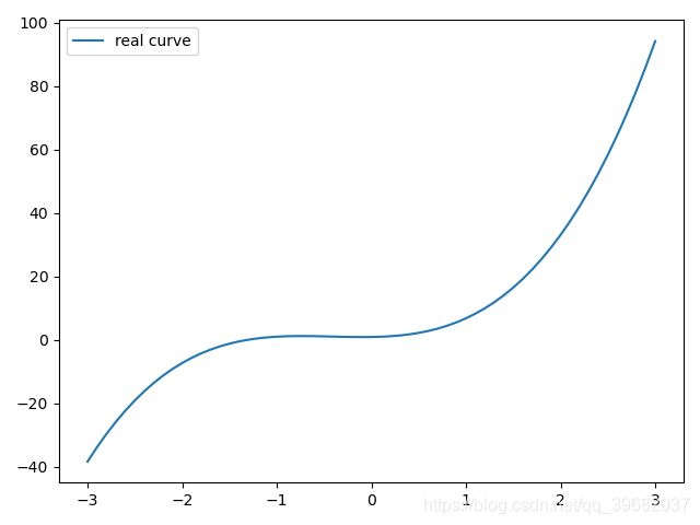
多项式回归模型
首先构造初始数据(小编感觉这时候画图更清晰)
import torch
from torch.autograd import Variable


import numpy as np
import matplotlib.pyplot as plt


class LinearModel(object):
    def __init__(self):
        pass

    def mult(self):
        '''
        实现多项式线性回归
        :retrun: None
        '''

        # 定义权重w1,w2,w3 和 偏置b
        # y = 0.90 + 0.50 * x + 3.00 * x^2 + 2.40 * x^3
        w_target = np.array([0.5, 3, 2.4])
        b_target = np.array([0.9])

        f_des = 'y = {:.2f} + {:.2f} * x + {:.2f} * x^2 + {:.2f} * x^3'.format(
            b_target[0], w_target[0], w_target[1], w_target[2])  # 打印出函数的式子

        print(f_des)

        # 画出这个函数的曲线
        x_sample = np.arange(-3, 3.1, 0.1)
        y_sample = b_target[0] + w_target[0] * x_sample + w_target[1] * x_sample ** 2 + w_target[2] * x_sample ** 3

        plt.plot(x_sample, y_sample, label='real curve')
        plt.legend()
        plt.show()

        return None


if __name__ == "__main__":
    model = LinearModel()
    model.mult()
    pass
画出没有更新之前的预测模型和真实的模型之间的对比
import torch
from torch.autograd import Variable


import numpy as np
import matplotlib.pyplot as plt


class LinearModel(object):
    def __init__(self):
        pass

    def mult(self):
        '''
        实现多项式线性回归
        :retrun: None
        '''

        # 定义权重w1,w2,w3 和 偏置b
        # y = 0.90 + 0.50 * x + 3.00 * x^2 + 2.40 * x^3
        w_target = np.array([0.5, 3, 2.4])
        b_target = np.array([0.9])

        f_des = 'y = {:.2f} + {:.2f} * x + {:.2f} * x^2 + {:.2f} * x^3'.format(
            b_target[0], w_target[0], w_target[1], w_target[2])  # 打印出函数的式子

        print(f_des)


        x_sample = np.arange(-3, 3.1, 0.1)
        y_sample = b_target[0] + w_target[0] * x_sample + w_target[1] * x_sample ** 2 + w_target[2] * x_sample ** 3
        # # 画出这个函数的曲线
        # plt.plot(x_sample, y_sample, label='real curve')
        # plt.legend()
        # plt.show()

        # 构建数据 x 和 y
        # x 是一个如下矩阵 [x, x^2, x^3]
        # y 是函数的结果 [y]

        x_train = np.stack([x_sample ** i for i in range(1, 4)], axis=1)
        x_train = torch.from_numpy(x_train).float()  # 转换成 float tensor

        y_train = torch.from_numpy(y_sample).float().unsqueeze(1)  # 转化成 float tensor

        # 定义参数和模型
        w = Variable(torch.randn(3, 1), requires_grad=True)
        b = Variable(torch.zeros(1), requires_grad=True)

        # 将 x 和 y 转换成 Variable
        x_train = Variable(x_train)
        y_train = Variable(y_train)

        # 做出预测
        y_predict = torch.mm(x_train,w)+b

        # 画出没有更新之前的模型和真实的模型之间的对比
        plt.plot(x_train.data.numpy()[:, 0], y_predict.data.numpy(), label='fitting curve', color='r')
        plt.plot(x_train.data.numpy()[:, 0], y_sample, label='real curve', color='b')
        plt.legend()
        plt.show()


        return None


if __name__ == "__main__":
    model = LinearModel()
    model.mult()
    pass

发现更新完成之后 loss 慢慢变小了,经过100次训练,两条线近乎重合
import torch
from torch.autograd import Variable


import numpy as np
import matplotlib.pyplot as plt


class LinearModel(object):
    def __init__(self):
        pass
    def get_loss(self,y_predict,y_train):
        '''
        计算损失
        :param y_predict 预测值
        :param y_train 训练值
        :return: 误差
        '''
        return torch.mean((y_predict - y_train) ** 2 )
    def mult(self):
        '''
        实现多项式线性回归
        :retrun: None
        '''

        # 定义权重w1,w2,w3 和 偏置b
        # y = 0.90 + 0.50 * x + 3.00 * x^2 + 2.40 * x^3
        w_target = np.array([0.5, 3, 2.4])
        b_target = np.array([0.9])

        f_des = 'y = {:.2f} + {:.2f} * x + {:.2f} * x^2 + {:.2f} * x^3'.format(
            b_target[0], w_target[0], w_target[1], w_target[2])  # 打印出函数的式子

        print(f_des)


        x_sample = np.arange(-3, 3.1, 0.1)
        y_sample = b_target[0] + w_target[0] * x_sample + w_target[1] * x_sample ** 2 + w_target[2] * x_sample ** 3
        # # 画出这个函数的曲线
        # plt.plot(x_sample, y_sample, label='real curve')
        # plt.legend()
        # plt.show()

        # 构建数据 x 和 y
        # x 是一个如下矩阵 [x, x^2, x^3]
        # y 是函数的结果 [y]

        x_train = np.stack([x_sample ** i for i in range(1, 4)], axis=1)
        x_train = torch.from_numpy(x_train).float()  # 转换成 float tensor

        y_train = torch.from_numpy(y_sample).float().unsqueeze(1)  # 转化成 float tensor

        # 定义参数和模型
        w = Variable(torch.randn(3, 1), requires_grad=True)
        b = Variable(torch.zeros(1), requires_grad=True)

        # 将 x 和 y 转换成 Variable
        x_train = Variable(x_train)
        y_train = Variable(y_train)

        # 做出预测
        y_predict = torch.mm(x_train,w)+b

        # # 画出没有更新之前的模型和真实的模型之间的对比
        # plt.plot(x_train.data.numpy()[:, 0], y_predict.data.numpy(), label='fitting curve', color='r')
        # plt.plot(x_train.data.numpy()[:, 0], y_sample, label='real curve', color='b')
        # plt.legend()
        # plt.show()

        # 计算误差
        loss = self.get_loss(y_predict,y_train)

        print(loss)

        # 自动求导
        loss.backward()

        # 查看一下 w 和 b 的梯度
        print(w.grad)
        print(b.grad)

        # 进行 100 次参数更新
        for e in range(100):
            y_pred = torch.mm(x_train,w)+b
            loss = self.get_loss(y_pred, y_train)

            w.grad.data.zero_()
            b.grad.data.zero_()
            loss.backward()

            # 更新参数
            w.data = w.data - 0.001 * w.grad.data
            b.data = b.data - 0.001 * b.grad.data
            if (e + 1) % 20 == 0:
                print('epoch {}, Loss: {:.5f}'.format(e + 1, loss))

        # 画出更新一次之后的模型
        y_pred = torch.mm(x_train,w)+b

        plt.plot(x_train.data.numpy()[:, 0], y_pred.data.numpy(), label='fitting curve', color='r')
        plt.plot(x_train.data.numpy()[:, 0], y_sample, label='real curve', color='b')
        plt.legend()
        plt.show()


        return None


if __name__ == "__main__":
    model = LinearModel()
    model.mult()
    pass

