【深度学习笔记】03 微积分与自动微分

导数和微分

假设我们有一个函数$f:\mathbb{R}\to \mathbb{R}$，其输入和输出都是标量。
如果$f$的导数存在，这个极限被定义为

$$f^{\prime }(x)=\underset{h\to 0}{\lim }\frac{f(x+h)-f(x)}{h}.$$

如果$f^{\prime }(a)$存在，则称$f$在$a$处是可微（differentiable）的。
如果$f$在一个区间内的每个数上都是可微的，则此函数在此区间中是可微的。
我们可以将导数$f^{\prime }(x)$解释为$f(x)$相对于$x$的瞬时（instantaneous）变化率。
所谓的瞬时变化率是基于$x$中的变化$h$，且$h$接近$0$。

给定$y=f(x)$，其中$x$和$y$分别是函数$f$的自变量和因变量。以下表达式是等价的：

$$f^{\prime }(x)=y^{\prime }=\frac{dy}{dx}=\frac{df}{dx}=\frac{d}{dx}f(x)=Df(x)=D_{x}f(x),$$

其中符号$\frac{d}{dx}$和$D$是微分运算符，表示微分操作。
可以使用以下规则来对常见函数求微分：

• $DC=0$（$C$是一个常数）
• $D{x}^n=n{x}^{n-1}$（幂律（power rule），$n$是任意实数）
• $D{e}^x=e^x$
• $D\ln (x)=1/x$

假设函数$f$和$g$都是可微的，$C$是一个常数，则：

常数相乘法则
$$\frac{d}{dx}[Cf(x)]=C\frac{d}{dx}f(x),$$

加法法则

$$\frac{d}{dx}[f(x)+g(x)]=\frac{d}{dx}f(x)+\frac{d}{dx}g(x),$$

乘法法则

$$\frac{d}{dx}[f(x)g(x)]=f(x)\frac{d}{dx}[g(x)]+g(x)\frac{d}{dx}[f(x)],$$

除法法则

$$\frac{d}{dx}\left[\frac{f(x)}{g(x)}\right]=\frac{g(x)\frac{d}{dx}[f(x)]-f(x)\frac{d}{dx}[g(x)]}{[g(x){]}^2}.$$

导数解释的可视化

import numpy as np
from matplotlib_inline import backend_inline
from d2l import torch as d2l

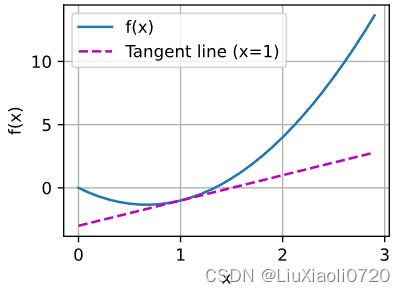
def f(x):
    return 3 * x ** 2 - 4 * x

def use_svg_display():  #@save
    """使用svg格式在Jupyter中显示绘图"""
    backend_inline.set_matplotlib_formats('svg')

定义set_figsize函数来设置图表大小

def set_figsize(figsize=(3.5, 2.5)):  #@save
    """设置matplotlib的图表大小"""
    use_svg_display()
    d2l.plt.rcParams['figure.figsize'] = figsize

set_axes函数用于设置由matplotlib生成图表的轴的属性

#@save
def set_axes(axes, xlabel, ylabel, xlim, ylim, xscale, yscale, legend):
    """设置matplotlib的轴"""
    axes.set_xlabel(xlabel)
    axes.set_ylabel(ylabel)
    axes.set_xscale(xscale)
    axes.set_yscale(yscale)
    axes.set_xlim(xlim)
    axes.set_ylim(ylim)
    if legend:
        axes.legend(legend)
    axes.grid()

通过这三个用于图形配置的函数，定义一个plot函数来简洁地绘制多条曲线。

#@save
def plot(X, Y=None, xlabel=None, ylabel=None, legend=None, xlim=None,
         ylim=None, xscale='linear', yscale='linear',
         fmts=('-', 'm--', 'g-.', 'r:'), figsize=(3.5, 2.5), axes=None):
    """绘制数据点"""
    if legend is None:
        legend = []

    set_figsize(figsize)
    axes = axes if axes else d2l.plt.gca()

    # 如果X有一个轴，输出True
    def has_one_axis(X):
        return (hasattr(X, "ndim") and X.ndim == 1 or isinstance(X, list)
                and not hasattr(X[0], "__len__"))

    if has_one_axis(X):
        X = [X]
    if Y is None:
        X, Y = [[]] * len(X), X
    elif has_one_axis(Y):
        Y = [Y]
    if len(X) != len(Y):
        X = X * len(Y)
    axes.cla()
    for x, y, fmt in zip(X, Y, fmts):
        if len(x):
            axes.plot(x, y, fmt)
        else:
            axes.plot(y, fmt)
    set_axes(axes, xlabel, ylabel, xlim, ylim, xscale, yscale, legend)

绘制函数$u=f(x)$及其在$x=1$处的切线$y=2x-3$，其中系数$2$是切线的斜率

x = np.arange(0, 3, 0.1)
plot(x, [f(x), 2 * x - 3], 'x', 'f(x)', legend=['f(x)', 'Tangent line (x=1)'])

​

​

偏导数

设$y=f(x_1,x_2,\dots ,x_n)$是一个具有$n$个变量的函数。
$y$关于第$i$个参数$x_i$的偏导数（partial derivative）为：
​
$$\frac{\partial y}{\partial x_i}=\underset{h\to 0}{\lim }\frac{f(x_1,\dots ,x_{i-1},x_i+h,x_{i+1},\dots ,x_n)-f(x_1,\dots ,x_i,\dots ,x_n)}{h}.$$
​
为了计算$\frac{\partial y}{\partial x_i}$，
可以将$x_1,\dots ,x_{i-1},x_{i+1},\dots ,x_n$看作常数，
并计算$y$关于$x_i$的导数。
对于偏导数的表示，以下是等价的：
​
$$\frac{\partial y}{\partial x_i}=\frac{\partial f}{\partial x_i}=f_{x_i}=f_i=D_{i}f=D_{x_i}f.$$
​

梯度

可以连结一个多元函数对其所有变量的偏导数，以得到该函数的梯度（gradient）向量。
设函数$f:{\mathbb{R}}^n\to \mathbb{R}$的输入是
一个$n$维向量$\mathbf{x}=[x_1,x_2,\dots ,x_n{]}^{\top }$，并且输出是一个标量。
函数$f(\mathbf{x})$相对于$\mathbf{x}$的梯度是一个包含$n$个偏导数的向量:
​
$${\nabla }_{\mathbf{x}}f(\mathbf{x})=[\frac{\partial f(\mathbf{x})}{\partial x_1},\frac{\partial f(\mathbf{x})}{\partial x_2},\dots ,\frac{\partial f(\mathbf{x})}{\partial x_n}{]}^{\top },$$
​
其中${\nabla }_{\mathbf{x}}f(\mathbf{x})$通常在没有歧义时被$\nabla f(\mathbf{x})$取代。
​
假设$\mathbf{x}$为$n$维向量，在微分多元函数时经常使用以下规则:
​

• 对于所有$\mathbf{A}\in {\mathbb{R}}^{m\times n}$，都有${\nabla }_{\mathbf{x}}\mathbf{Ax}={\mathbf{A}}^{\top }$
• 对于所有$\mathbf{A}\in {\mathbb{R}}^{n\times m}$，都有${\nabla }_{\mathbf{x}}{\mathbf{x}}^{\top }\mathbf{A}=\mathbf{A}$
• 对于所有$\mathbf{A}\in {\mathbb{R}}^{n\times n}$，都有${\nabla }_{\mathbf{x}}{\mathbf{x}}^{\top }\mathbf{Ax}=(\mathbf{A}+{\mathbf{A}}^{\top })\mathbf{x}$
• ${\nabla }_{\mathbf{x}}\Vert \mathbf{x}{\Vert }^2={\nabla }_{\mathbf{x}}{\mathbf{x}}^{\top }\mathbf{x}=2\mathbf{x}$
  ​
  同样，对于任何矩阵$\mathbf{X}$，都有${\nabla }_{\mathbf{X}}\Vert \mathbf{X}{\Vert }_F^2=2\mathbf{X}$。

链式法则

链式法则可以被用来微分复合函数。
​
假设函数$y=f(u)$和$u=g(x)$都是可微的，根据链式法则：
​
$$\frac{dy}{dx}=\frac{dy}{du}\frac{du}{dx}.$$
​
现在考虑一个更一般的场景，即函数具有任意数量的变量的情况。
假设可微分函数$y$有变量$u_1,u_2,\dots ,u_m$，其中每个可微分函数$u_i$都有变量$x_1,x_2,\dots ,x_n$。
注意，$y$是$x_1,x_2，\dots ,x_n$的函数。
对于任意$i=1,2,\dots ,n$，链式法则给出：
​
$$\frac{\partial y}{\partial x_i}=\frac{\partial y}{\partial u_1}\frac{\partial u_1}{\partial x_i}+\frac{\partial y}{\partial u_2}\frac{\partial u_2}{\partial x_i}+\cdots +\frac{\partial y}{\partial u_m}\frac{\partial u_m}{\partial x_i}$$
​

自动微分

深度学习框架通过自动计算导数，即自动微分（automatic differentiation）来加快求导。
实际中，根据设计好的模型，系统会构建一个计算图（computational graph），
来跟踪计算是哪些数据通过哪些操作组合起来产生输出。
自动微分使系统能够随后反向传播梯度。
这里，反向传播（backpropagate）意味着跟踪整个计算图，填充关于每个参数的偏导数。

例如对函数$y=2x^{T}x$关于列向量$x$求导

首先创建变量$x$并为其分配一个初始值

import torch

x = torch.arange(4.0)
x

tensor([0., 1., 2., 3.])

x.requires_grad_(True)  # 等价于x=torch.arange(4.0,requires_grad=True)
x.grad  # 默认值是None

# 计算y
y = 2 * torch.dot(x, x)
y

tensor(28., grad_fn=)

通过调用反向传播函数来自动计算$y$关于$x$每个分量的梯度

y.backward()
x.grad

tensor([ 0.,  4.,  8., 12.])

验证梯度计算是否正确

x.grad == 4 * x

tensor([True, True, True, True])

计算$x$的另一个函数

# 在默认情况下，PyTorch会累计梯度，需要清除之前的值
x.grad.zero_()
y = x.sum()
y.backward()
x.grad

tensor([1., 1., 1., 1.])

非标量变量的反向传播

# 对非标量调用backward需要传入一个gradient参数，该参数指定微分函数关于self的梯度。
# 本例只想求偏导数的和，所以传递一个1的梯度是合适的
x.grad.zero_()
y = x * x
# 等价于y.backward(torch.ones(len(x)))
y.sum().backward()
x.grad

tensor([0., 2., 4., 6.])

分离计算

有时希望将某些计算移动到记录的计算图之外。例如，加入$y$是作为$x$的函数计算的，而$z$则是作为$y$和$x$的函数计算的。此时想计算$z$关于$x$的梯度，但由于某种原因，希望将$y$视为一个常熟，并且只考虑到$x$在$y$被计算之后发挥的作用。

这里可以分离$y$来返回一个新变量$u$，该变量与$y$具有相同的值，但丢弃计算图中如何计算$y$的任何信息，即梯度不会向后流经$u$到$x$。

因此，反向传播函数计算$z=u\ast x$关于$x$的偏导数，同时将$u$作为常数处理，而不是$z=x\ast x\ast x$关于$x$的偏导数。

x.grad.zero_()
y = x * x
u = y.detach()
z = u * x

z.sum().backward()
x.grad == u

tensor([True, True, True, True])

由于记录了$y$的计算结果，我们随后可以在$y$上调用反向传播，得到$y=x\ast x$关于$x$的导数，即$2\ast x$

x.grad.zero_()
y.sum().backward()
x.grad == 2 * x

tensor([True, True, True, True])