Using Python to Simulate Brownian Motion
Brownian motion is a phenomenon that particles in the seemingly motionless liquid are still undergone unceasing collisions in an erratic way. It was firstly observed by Robert Brown in 1827. In 1923, Norbert Wiener had attempted to formulate this observations in mathematical terms; thus it is also known as Wiener process.
Owing to its randomness, Brownian motion has a wide range of applications, ranging from chaotic oscillations to stock market fluctuations. In this article, I will describe its basic property and how to visualise it and its variants with Python.
The Model of Brownian Motion
To begin with, we should see how to make Brownian motion in a rather formal way.
We firstly consider one dimensional coordinate system for simplicity. Imagine that you put a particle at the origin (x=0) in the very beginning, and it may encounter random collisions along the x-coordinate afterwards. Let X ( t ) X(t) X(t) be the position of the particle after t t t units of time ( X ( 0 ) = 0 X(0)=0 X(0)=0).
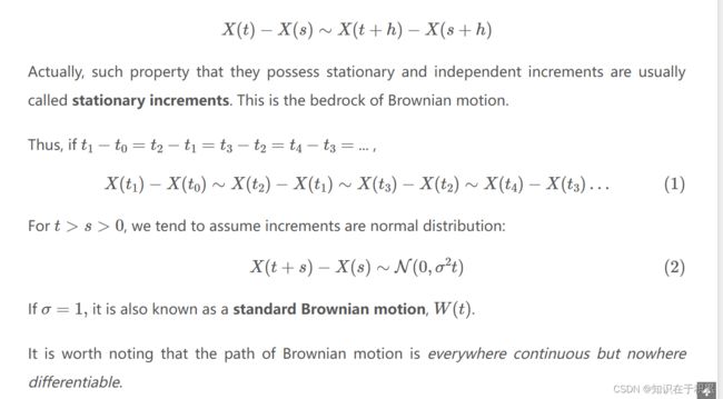
When the particle is undergone some collisions, we say there are events occurred. From physical obervations, scientists find that the probability of events occurred in any two equal time intervals, say [x,t]
and [x+h,t+h], are not only equal but also indepedent. In other words, they have the same probability distribution, and no matter how many events occurred in [x,t], it would not affect the number of events occurred over [x+h,t+h]. This can be represented as
Visualise the Brownian Motion
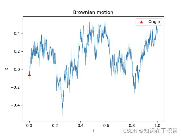
Now we are ready to draw our Brownian motion in Python.
Some Toolkits
Below are the modules we will use to draw our plots.
from math import sqrt, exp
from random import random, gauss
import numpy as np
import matplotlib.pyplot as plt
Visualisation
mean = 0
std = random()  # standard deviation

N = 1000    # generate N points
dt = 1/N    # time interval = [0,1]

data = []
x = 0
for t in range(N):
    dx = gauss(mean, std*sqrt(dt))  # gauss(mean, standard deviation)
    x = x + dx                      # compute X(t) incrementally
    data.append((dt*t, x+dx))

data = np.array(data)

plt.figure()
plt.plot(data[:, 0], data[:, 1], linewidth=0.5)
plt.scatter(data[0, 0], data[0, 1],marker="^",color='r',label="Origin")
plt.xlabel('t')
plt.ylabel('x')
plt.legend()
plt.title("Brownian motion")
plt.show()
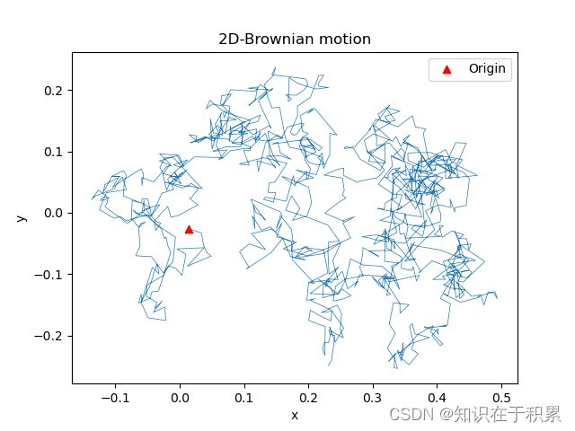
2D-Brownian Motion
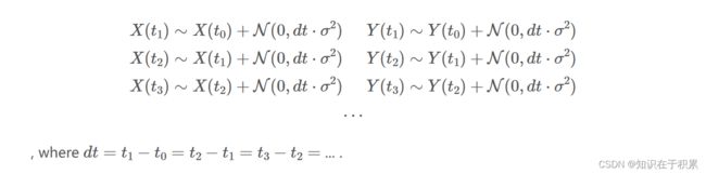
Similarly, if we extend our coordinate system to two dimensions,
mean = 0
std = random()

N = 1000    # generate N points
dt = 1/N    # time interval = [0,1]

data = []
x, y = 0, 0
for t in range(N):
    dx = gauss(mean, std*sqrt(dt))
    dy = gauss(mean, std*sqrt(dt))
    x, y = x+dx, y+dy
    data.append((x, y))

data = np.array(data)

plt.figure()
plt.plot(data[:, 0], data[:, 1], linewidth=0.5)
plt.scatter(data[0, 0], data[0, 1],marker="^",color='r',label="Origin")
plt.xlabel('x')
plt.ylabel('y')
plt.legend()
plt.title("2D-Brownian motion")
plt.show()
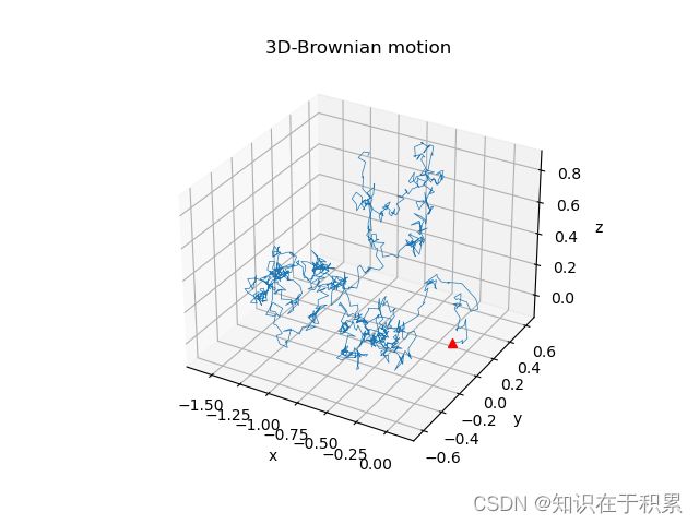
3D-Brownian Motion
The Brownian motion over 3-dim coordinate system is also trivial when you grasp the idea.
mean = 0
std = random()  # standard deviation

N = 1000    # generate N points
dt = 1/N    # time interval = [0,1]

data = []
x, y, z = 0, 0, 0
for t in range(N):
    dx = gauss(mean, std*sqrt(dt))
    dy = gauss(mean, std*sqrt(dt))
    dz = gauss(mean, std*sqrt(dt))
    x, y, z = x+dx, y+dy, z+dz
    data.append((x, y, z))

data = np.array(data)

plt.figure()
ax = plt.axes(projection='3d')
ax.plot3D(data[:, 0], data[:, 1], data[:, 2], linewidth=0.5)
ax.plot3D(data[0, 0], data[0, 1], data[0, 2], marker='^', color='r')
ax.set_xlabel('x')
ax.set_ylabel('y')
ax.set_zlabel('z')
ax.set_title('3D-Brownian motion')
plt.show()
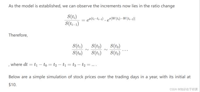
Geometric Brownian Motion
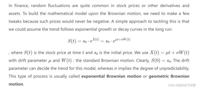
The Relationship between Stock Prices at Time t
mean = random()
std = random()

N = 253     # trading days in a year
dt = 1/N

x = 10.0    # initial stock price
data = [(0, x)]
for t in range(1, N):
    ratio = exp(mean*dt) * exp(std * gauss(0, sqrt(dt)))
    x = x * ratio
    data.append((dt*t, x))

data = np.array(data)

plt.figure()
plt.plot(data[:, 0], data[:, 1], linewidth=0.5)
plt.plot(data[0, 0], data[0, 1], marker='^', color='r')
plt.xlabel('t')
plt.ylabel('price')
plt.ylim([0, max(data[:,1]+10)])
plt.title("Geometric Brownian motion")
plt.show()

See https://lucien-east.github.io/2021/07/27/Brownian-motion/