DNN二分类模型

import os
import datetime

#打印时间
def printbar():
    nowtime = datetime.datetime.now().strftime('%Y-%m-%d %H:%M:%S')
    print("\n"+"=========="*8 + "%s"%nowtime)

#mac系统上pytorch和matplotlib在jupyter中同时跑需要更改环境变量
os.environ["KMP_DUPLICATE_LIB_OK"]="TRUE" 
printbar()

准备数据：

import numpy as np 
import pandas as pd 
from matplotlib import pyplot as plt
import torch
from torch import nn
%matplotlib inline
%config InlineBackend.figure_format = 'svg'

#正负样本数量
n_positive,n_negative = 2000,2000

#生成正样本, 小圆环分布              torch.normal 是 PyTorch 的一个函数，用于根据正态分布（高斯分布）生成随机数张量
r_p = 5.0 + torch.normal(0.0,1.0,size = [n_positive,1])   # 0.0表示均值，1.0表示标准差的正态分布， torch.normal(mean, std, size)
#print(r_p.shape)
theta_p = 2*np.pi*torch.rand([n_positive,1])  #torch.rand 是 PyTorch 中用于生成均匀分布（uniform distribution）的随机数张量的函数
# torch.rand()生成0到之间的均匀分布的随机数，torch.normal生成指定均值和标准差的正太分布的随机数
#print(theta_p.shape)   theta_p形状是[2000,1],每个数范围是0到2Π，cos(theta_p)范围是余弦函数一个周期的图像，*r_p表示（rcos角度，rsin角度）
Xp = torch.cat([r_p*torch.cos(theta_p),r_p*torch.sin(theta_p)],axis = 1)
# torch.cat 拼接两个生成一个二维张量，axis = 1表示在axis = 1方向上拼接，就是Xp（x,y）坐标，x,y都是-5到5之内的数，Xp的每一行表示一个点
print(Xp.shape)
Yp = torch.ones_like(r_p)
print(Yp.shape)

#生成负样本, 大圆环分布
r_n = 8.0 + torch.normal(0.0,1.0,size = [n_negative,1]) 
theta_n = 2*np.pi*torch.rand([n_negative,1])
Xn = torch.cat([r_n*torch.cos(theta_n),r_n*torch.sin(theta_n)],axis = 1)
Yn = torch.zeros_like(r_n)

#汇总样本
X = torch.cat([Xp,Xn],axis = 0)   # 正负样本所有点进行拼接。在0维度上，也就是把两个n行，每行一系列点的张量在行上往下拼接
Y = torch.cat([Yp,Yn],axis = 0)   # Yp,Yn表示正负样本的标签，也就是二分类的类别标签而已
 

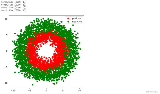
#可视化
plt.figure(figsize = (6,6))
plt.scatter(Xp[:,0].numpy(),Xp[:,1].numpy(),c = "r")
plt.scatter(Xn[:,0].numpy(),Xn[:,1].numpy(),c = "g")
plt.legend(["positive","negative"]);

# 构建数据管道迭代器
def data_iter(features, labels, batch_size=8):
    num_examples = len(features)  #样本总个数，就是点的总个数  len()函数来获取列表的长度，也就是样本的数量
    indices = list(range(num_examples))  # 转换成列表类型  range(num_examples)生成一个有序数组，转成列表形式，
    # Python中，range()函数生成的整数序列范围为 [start, end) (包左不包右)
    # torch.range()函数生成的整数序列范围为 [start, end] (包左包右) 
    np.random.shuffle(indices)  #样本的读取顺序是随机的，打乱样本点的索引
    for i in range(0, num_examples, batch_size):
        # 列表切片，根据样本个数长度范围内的随机列表生成一个批次的列表索引
        indexs = torch.LongTensor(indices[i: min(i + batch_size, num_examples)])   
        # features输入的是X，[4000,2]的4000个点的张量格式，
        # torch.index_select是PyTorch中的一个函数，其主要用途是允许您在特定维度上选择索引，从而获取所需的张量子集2。
        yield  features.index_select(0, indexs), labels.index_select(0, indexs)  # 取出总样本中batch_size个数据
        
# 测试数据管道效果   
batch_size = 8
# X,Y 是正负样本也就是两个类别拼接后的张量，X是点，Y是点的类别
(features,labels) = next(data_iter(X,Y,batch_size))
print(features)
print(labels)

class DNNModel(nn.Module):
    def __init__(self):
        super(DNNModel, self).__init__()
        self.w1 = nn.Parameter(torch.randn(2,4))  # 两行四列
        self.b1 = nn.Parameter(torch.zeros(1,4))  # 偏置全是0
        self.w2 = nn.Parameter(torch.randn(4,8))
        self.b2 = nn.Parameter(torch.zeros(1,8))
        self.w3 = nn.Parameter(torch.randn(8,1))
        self.b3 = nn.Parameter(torch.zeros(1,1))   # 最后预测结果形状[8,1]  是8个数的大小，就是这组权重偏置预测出来的结果

    # 正向传播
    def forward(self,x):
        x = torch.relu([email protected] + self.b1)
        x = torch.relu([email protected] + self.b2)
        y = torch.sigmoid([email protected] + self.b3)
        return y   # y就是预测
    
    # 损失函数(二元交叉熵)
    def loss_fn(self,y_pred,y_true):  
        #将预测值限制在1e-7以上, 1- (1e-7)以下，避免log(0)错误
        eps = 1e-7
        y_pred = torch.clamp(y_pred,eps,1.0-eps)
        bce = - y_true*torch.log(y_pred) - (1-y_true)*torch.log(1-y_pred)
        return torch.mean(bce)
    
    # 评估指标(准确率)
    def metric_fn(self,y_pred,y_true):
        y_pred = torch.where(y_pred>0.5,torch.ones_like(y_pred,dtype = torch.float32),
                          torch.zeros_like(y_pred,dtype = torch.float32))
        acc = torch.mean(1-torch.abs(y_true-y_pred))
        return acc
    
model = DNNModel()

# 测试模型结构
batch_size = 10
(features,labels) = next(data_iter(X,Y,batch_size))

predictions = model(features)

loss = model.loss_fn(labels,predictions)
metric = model.metric_fn(labels,predictions)

print("init loss:", loss.item())
print("init metric:", metric.item())

训练模型

def train_step(model, features, labels):   
    
    # 正向传播求损失
    predictions = model.forward(features)
    loss = model.loss_fn(predictions,labels)
    metric = model.metric_fn(predictions,labels)
        
    # 反向传播求梯度
    loss.backward()
    
    # 梯度下降法更新参数
    for param in model.parameters():
        #注意是对param.data进行重新赋值,避免此处操作引起梯度记录
        param.data = (param.data - 0.01*param.grad.data) 
        
    # 梯度清零
    model.zero_grad()
        
    return loss.item(),metric.item()
 

def train_model(model,epochs):
    for epoch in range(1,epochs+1):
        loss_list,metric_list = [],[]
        for features, labels in data_iter(X,Y,20):
            # 分批训练
            lossi,metrici = train_step(model,features,labels)
            loss_list.append(lossi)
            metric_list.append(metrici)
        loss = np.mean(loss_list)
        metric = np.mean(metric_list)

        if epoch%10==0:
            printbar()  # 最开始定义的打印时间的函数
            print("epoch =",epoch,"loss = ",loss,"metric = ",metric)
        
train_model(model,epochs = 100)

# 结果可视化
fig, (ax1,ax2) = plt.subplots(nrows=1,ncols=2,figsize = (12,5))
ax1.scatter(Xp[:,0],Xp[:,1], c="r")
ax1.scatter(Xn[:,0],Xn[:,1],c = "g")
ax1.legend(["positive","negative"]);
ax1.set_title("y_true");

Xp_pred = X[torch.squeeze(model.forward(X)>=0.5)]
Xn_pred = X[torch.squeeze(model.forward(X)<0.5)]

ax2.scatter(Xp_pred[:,0],Xp_pred[:,1],c = "r")
ax2.scatter(Xn_pred[:,0],Xn_pred[:,1],c = "g")
ax2.legend(["positive","negative"]);
ax2.set_title("y_pred");