BikeDNA（三） OSM数据的内在分析2

BikeDNA（三） OSM数据的内在分析2

1.数据完整性

见上一篇BikeDNA（二） OSM数据的内在分析1

2.OSM标签分析

见上一篇BikeDNA（二） OSM数据的内在分析1

3.网络拓扑结构

本节探讨数据的几何和拓扑特征。 例如，这些是网络密度、断开的组件和悬空（一级）节点。 它还包括探索是否存在彼此非常接近但不共享边缘的节点（边缘下冲的潜在迹象），或者是否存在相交边缘而在相交处没有节点，这可能表明存在数字化错误，该错误将导致数字化错误。 扭曲网络上的路由。

由于大多数自行车网络的分散性，许多指标（例如缺失链接或网络间隙）可以简单地反映基础设施的真实范围(Natera Orozco et al., 2020)。 这对于道路网络来说是不同的，例如，断开的组件更容易被解释为数据质量问题。 因此，分析仅将非常小的网络间隙视为潜在的数据质量问题。

3.1 简化结果

为了比较网络中节点和边之间的结构和真实比率，通过删除所有间隙节点，在笔记本“1a”中创建了仅包括端点和交叉点处的节点的简化网络表示。

比较简化前后网络的度分布是对简化例程的快速健全性检查。 通常，非简化网络中的绝大多数节点都是二级节点； 然而，在简化的网络中，大多数节点的度数不是二。 仅在两种情况下保留二级节点：如果它们代表两种不同类型的基础设施之间的连接点； 或者如果需要它们以避免自环（起点和终点相同的边）或同一对节点之间的多个边。

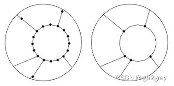
非简化网络（左）和简化网络（右）。

方法

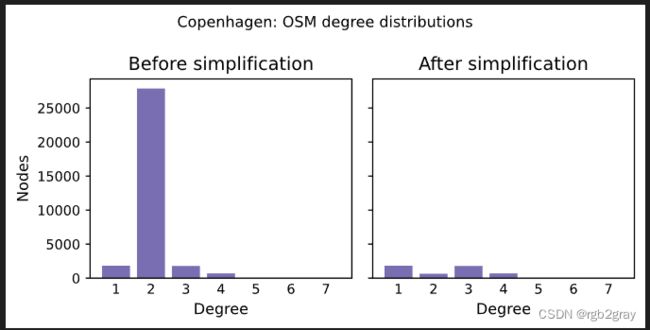
简化前后的度分布如下图所示。

解释

通常，度分布将从高（简化前）到低（简化后）二度节点计数，而对于所有其他度（1 或 3 及更高），它不会改变。 此外，节点总数将出现大幅下降。 如果简化后的图仍然保持相对较高的二度节点数量，或者简化后具有其他度数的节点数量发生变化，则这可能表明图转换或简化过程存在问题。

# Decrease in network elements after simplification

edge_percent_diff = (len(osm_edges) - len(osm_edges_simplified)) / len(osm_edges) * 100
node_percent_diff = (len(osm_nodes) - len(osm_nodes_simplified)) / len(osm_nodes) * 100

simplification_results = {
    "edge_percent_diff": edge_percent_diff,
    "node_percent_diff": node_percent_diff,
}

print(
    f"Simplifying the network decreased the number of edges by {edge_percent_diff:.1f}% and the number of nodes by {node_percent_diff:.1f}%."
)

Simplifying the network decreased the number of edges by 89.0% and the number of nodes by 84.4%.

# Degree distribution

set_renderer(renderer_plot)
fig, ax = plt.subplots(1, 2, figsize=pdict["fsbar_short"], sharey=True)

degree_sequence_before = sorted((d for n, d in osm_graph.degree()), reverse=True)
degree_sequence_after = sorted(
    (d for n, d in osm_graph_simplified.degree()), reverse=True
)

# Plot degree distributions
ax[0].bar(*np.unique(degree_sequence_before, return_counts=True), tick_label = np.unique(degree_sequence_before), color=pdict["osm_base"])
ax[0].set_title("Before simplification")
ax[0].set_xlabel("Degree")
ax[0].set_ylabel("Nodes")

ax[1].bar(*np.unique(degree_sequence_after, return_counts=True), tick_label = np.unique(degree_sequence_after), color=pdict["osm_base"])
ax[1].set_title("After simplification")
ax[1].set_xlabel("Degree")

plt.suptitle(f"{area_name}: OSM degree distributions")

fig.tight_layout()

plot_func.save_fig(fig, osm_results_plots_fp + "degree_dist_osm")

plt.show();

3.2 悬空节点

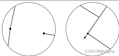
悬空节点是一阶节点，即它们仅附有一条边。 大多数网络自然会包含许多悬空节点。 悬空节点可能出现在实际的死胡同（代表死胡同）或某些特征的端点处，例如 当自行车道在街道中间结束时。 但是，在出现过冲/下冲的情况下，悬空节点也可能会作为数据质量问题出现（请参阅下一节）。 网络中悬空节点的数量在某种程度上也取决于数字化方法，如下图所示。

因此，悬空节点的存在本身并不是数据质量低的标志。 然而，在未知包含许多死胡同的区域中存在大量悬空节点可能表明数字化错误和边缘上冲/下冲问题。

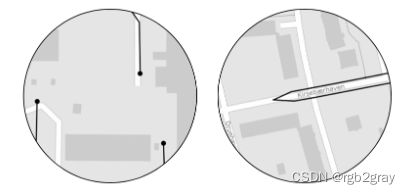
左：悬挂节点出现在道路要素结束处。 右：但是，当最后连接单独的特征时，将不会有悬空节点。 -->

左：悬挂节点出现在道路要素结束处。 右：但是，当最后连接单独的特征时，将不会有悬空节点。

方法

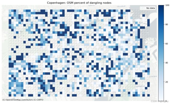
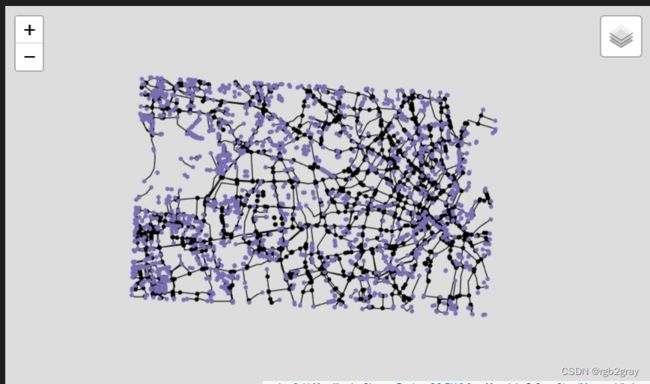
下面，在“get_dangling_nodes”的帮助下获得了所有悬空节点的列表。 然后，绘制包含所有节点的网络。 悬空节点以颜色显示，所有其他节点以黑色显示。

解释

我们建议进行可视化分析，以解释悬挂节点的空间分布，特别注意悬挂节点密度高的区域。 重要的是要了解悬挂节点的来源：它们是真正的死胡同还是数字化错误（例如，过冲/下冲）？ 数字化错误数量越多表明数据质量越低。

# Compute number of dangling nodes
dangling_nodes = eval_func.get_dangling_nodes(
    osm_edges_simplified, osm_nodes_simplified
)

# Export results
dangling_nodes.to_file(osm_results_data_fp + "dangling_nodes.gpkg", index=False)

# Compute local count and pct of dangling nodes
dn_osm_joined = gpd.overlay(
    dangling_nodes, grid[["geometry", "grid_id"]], how="intersection"
)
df = eval_func.count_features_in_grid(dn_osm_joined, "osm_dangling_nodes")
grid = eval_func.merge_results(grid, df, "left")

grid["osm_dangling_nodes_pct"] = np.round(
    100 * grid.count_osm_dangling_nodes / grid.count_osm_simplified_nodes, 2
)

# set to zero where there are simplified nodes but no dangling nodes
grid["osm_dangling_nodes_pct"].loc[
    grid.count_osm_simplified_nodes.notnull() & grid.osm_dangling_nodes_pct.isnull()
] = 0

# Plot dangling nodes

set_renderer(renderer_map)
fig, ax = plt.subplots(1, figsize=pdict["fsmap"])

from mpl_toolkits.axes_grid1 import make_axes_locatable
divider = make_axes_locatable(ax)
cax = divider.append_axes("right", size="3.5%", pad="1%")

grid.plot(
    cax=cax,
    column="osm_dangling_nodes_pct",
    ax=ax,
    alpha=pdict["alpha_grid"],
    cmap=pdict["pos"],
    legend=True,
)

# add no data patches
grid[grid["count_osm_simplified_nodes"].isnull()].plot(
    cax=cax,
    ax=ax,
    facecolor=pdict["nodata_face"],
    edgecolor=pdict["nodata_edge"],
    linewidth= pdict["line_nodata"],
    hatch=pdict["nodata_hatch"],
    alpha=pdict["alpha_nodata"],
)

ax.legend(handles=[nodata_patch], loc="upper right")
ax.set_title(f"{area_name}: OSM percent of dangling nodes")
ax.set_axis_off()
cx.add_basemap(ax=ax, crs=study_crs, source=cx_tile_2)

plot_func.save_fig(fig, osm_results_static_maps_fp + "pct_dangling_nodes_osm")

# Interactive plot of dangling nodes

edges_simplified_folium = plot_func.make_edgefeaturegroup(
    gdf=osm_edges_simplified,
    mycolor=pdict["base"],
    myweight=pdict["line_base"],
    nametag="Edges",
    show_edges=True,
)

nodes_simplified_folium = plot_func.make_nodefeaturegroup(
    gdf=osm_nodes_simplified,
    mysize=pdict["mark_base"],
    mycolor=pdict["base"],
    nametag="All nodes",
    show_nodes=True,
)

dangling_nodes_folium = plot_func.make_nodefeaturegroup(
    gdf=dangling_nodes,
    mysize=pdict["mark_emp"],
    mycolor= pdict["osm_base"],
    nametag="Dangling nodes",
    show_nodes=True,
)

m = plot_func.make_foliumplot(
    feature_groups=[
        edges_simplified_folium,
        nodes_simplified_folium,
        dangling_nodes_folium,
    ],
    layers_dict=folium_layers,
    center_gdf=osm_nodes_simplified,
    center_crs=osm_nodes_simplified.crs,
)

bounds = plot_func.compute_folium_bounds(osm_nodes_simplified)
m.fit_bounds(bounds)

m.save(osm_results_inter_maps_fp + "danglingmap_osm.html")

display(m)

print("Interactive map saved at " + osm_results_inter_maps_fp.lstrip("../") + "danglingmap_osm.html")

Interactive map saved at results/OSM/cph_geodk/maps_interactive/danglingmap_osm.html

3.3 下冲/过冲

当简化网络中的两个节点放置在几米距离内但不共享公共边缘时，通常是由于边缘上冲/下冲或其他数字化错误造成的。 当两个特征应该相交，但实际上彼此非常接近时，就会发生下冲。 当两个特征相遇并且其中一个特征超出另一个特征时，就会发生超调。 请参见下图的说明。 有关过冲/下冲的更详细说明，请参阅 GIS Lounge 网站。

左：当两条线要素未正确连接时（例如在交叉点处），会发生下冲。 右图：过冲是指线要素在相交线处延伸太远，而不是在相交处结束的情况。

方法

*下冲：*首先，“length_tolerance”（以米为单位）在下面的单元格中定义。 然后，使用“find_undershoots”，所有之间距离最大为“length_tolerance”的悬空节点对都被识别为下冲，并绘制结果。

*超调：*首先，“长度公差”（以米为单位）在下面的单元格中定义。 然后，使用“find_overshoots”，所有连接有悬空节点且最大长度为“length_tolerance”的网络边都被识别为过冲，并绘制结果。

过冲/下冲检测方法的灵感来自于 Neis et al. (2012)。

解释

欠调/过调不一定总是数据质量问题 - 它们可能是网络状况或数字化策略的准确表示。 例如，自行车道可能在转弯后不久突然结束，从而导致超调。 受保护的自行车道有时会在 OSM 中数字化，因为在交叉口处中断，从而导致交叉口下冲。

过冲/下冲对数据质量影响的解释取决于上下文。 对于某些应用，例如路由，过冲并不构成特殊的挑战； 然而，鉴于它们扭曲了网络结构，它们可能会给网络分析等其他应用带来问题。 相反，下冲对于路线应用来说是一个严重的问题，特别是如果只考虑自行车基础设施的话。 它们还给网络分析带来了问题，例如对于任何基于路径的度量，例如大多数中心性度量，如介数中心性。

User configurations

在分析过冲和下冲时，用户可以修改过冲和下冲的长度公差。
例如，过冲的长度容差为 3 米，这意味着只有长度为 3 米或更小的边缘片段才被视为过冲。
下冲容差为 5 米，意味着只有 5 米或更小的间隙才被视为下冲。

# USER INPUT: LENGTH TOLERANCE FOR OVER- AND UNDERSHOOTS
length_tolerance_over = 3
length_tolerance_under = 3

for s in [length_tolerance_over, length_tolerance_under]:
    assert isinstance(s, int) or isinstance(s, float), print(
        "Settings must be integer or float values!"
    )

print(f"Running overshoot analysis with a tolerance threshold of {length_tolerance_over} m.")
print(f"Running undershoot analysis with a tolerance threshold of {length_tolerance_under} m.")

Running overshoot analysis with a tolerance threshold of 3 m.
Running undershoot analysis with a tolerance threshold of 3 m.

### Overshoots

overshoots = eval_func.find_overshoots(
    dangling_nodes,
    osm_edges_simplified,
    length_tolerance_over,
    return_overshoot_edges=True,
)

print(
    f"{len(overshoots)} potential overshoots were identified using a length tolerance of {length_tolerance_over} m."
)

### Undershoots
undershoot_dict, undershoot_nodes = eval_func.find_undershoots(
    dangling_nodes,
    osm_edges_simplified,
    length_tolerance_under,
    "edge_id",
    return_undershoot_nodes=True,
)

print(
    f"{len(undershoot_nodes)} potential undershoots were identified using a length tolerance of {length_tolerance_under} m."
)

8 potential overshoots were identified using a length tolerance of 3 m.
18 potential undershoots were identified using a length tolerance of 3 m.

# Save to csv

overshoots[["edge_id", "length"]].to_csv(
    osm_results_data_fp + f"overshoot_edges_{length_tolerance_over}.csv", header = ["edge_id", "length (m)"], index = False
)

pd.DataFrame(undershoot_nodes["osmid"].to_list(), columns=["node_id"]).to_csv(
    osm_results_data_fp + f"undershoot_nodes_{length_tolerance_under}.csv", index=False
)

# Interactive plot of under/overshoots

simplified_edges_folium = plot_func.make_edgefeaturegroup(
    gdf=osm_edges_simplified,
    mycolor=pdict["base"],
    myweight=pdict["line_base"],
    nametag="Edges",
    show_edges=True,
)

fg = [simplified_edges_folium]

if len(overshoots) > 0 or len(undershoot_nodes) > 0:

    if len(overshoots) > 0:

        overshoots_folium = plot_func.make_edgefeaturegroup(
            gdf=overshoots,
            mycolor=pdict["osm_contrast"],
            myweight=pdict["line_emp2"],
            nametag="Overshoots",
            show_edges=True,
        )

        fg.append(overshoots_folium)

    if len(undershoot_nodes) > 0:

        undershoot_nodes_folium = plot_func.make_nodefeaturegroup(
            gdf=undershoot_nodes,
            mysize=pdict["mark_emp"],
            mycolor=pdict["osm_contrast2"],
            nametag="Undershoot nodes",
            show_nodes=True,
        )

        fg.append(undershoot_nodes_folium)

    m = plot_func.make_foliumplot(
        feature_groups=fg,
        layers_dict=folium_layers,
        center_gdf=osm_nodes_simplified,
        center_crs=osm_nodes_simplified.crs,
    )

    bounds = plot_func.compute_folium_bounds(osm_nodes_simplified)
    m.fit_bounds(bounds)

    m.save(
        osm_results_inter_maps_fp
        + f"underovershoots_{length_tolerance_under}_{length_tolerance_over}_osm.html"
    )

    display(m)

if len(undershoot_nodes) == 0:
    print("There are no undershoots to plot.")
if len(overshoots) == 0:
    print("There are no overshoots to plot.")

if len(overshoots) > 0 or len(undershoot_nodes) > 0:
    print("Interactive map saved at " + osm_results_inter_maps_fp.lstrip("../") + f"underovershoots_{length_tolerance_under}_{length_tolerance_over}_osm.html")
else:
    print("There are no under/overshoots to plot.")

Interactive map saved at results/OSM/cph_geodk/maps_interactive/underovershoots_3_3_osm.html

3.4 缺少交叉点

当两条边相交而相交处没有节点时 - 并且如果两条边都没有标记为桥或隧道 - 则明确指示存在拓扑错误。

方法

首先，在“check_intersection”的帮助下，检查未标记为隧道或桥的每个边缘是否与网络的另一个边缘有任何“交叉”。 如果是这种情况，则该边将被标记为存在相交问题。 打印发现的相交问题的数量，并绘制结果以进行可视化分析。 该方法的灵感来自 Neis et al. (2012)。

解释

交叉点问题数量越多表明数据质量越低。 但是，建议在对该区域有一定了解的情况下对所有交叉口问题进行手动目视检查，以确定交叉口问题的根源并确认/纠正/拒绝它们。

Warning

这是该笔记本中计算量最大的操作。 它可能比所有其他部分花费的时间长几倍。

missing_nodes_edge_ids, edges_with_missing_nodes = eval_func.find_missing_intersections(
    osm_edges, "edge_id"
)

count_intersection_issues = (
    len(missing_nodes_edge_ids) / 2
)  # The number of issues is counted twice since both intersecting osm_edges are returned

print(
    f"{count_intersection_issues:.0f} place(s) appear to be missing an intersection node or a bridge/tunnel tag."
)

0 place(s) appear to be missing an intersection node or a bridge/tunnel tag.

# Save to csv

if count_intersection_issues > 0: 
    pd.DataFrame(data=missing_nodes_edge_ids, columns=["edge_id"]).to_csv(
        osm_results_data_fp + "edges_missing_intersections.csv", index=False
    )

# Interactive plot of intersection issues

if count_intersection_issues > 0:

    simplified_edges_folium = plot_func.make_edgefeaturegroup(
        gdf=osm_edges_simplified,
        mycolor=pdict["base"],
        myweight=pdict["line_base"],
        nametag="All edges",
        show_edges=True,
    )

    intersection_issues_folium = plot_func.make_edgefeaturegroup(
        gdf=edges_with_missing_nodes,
        mycolor=pdict["osm_contrast"],
        myweight=pdict["line_emp"],
        nametag="Intersection issues: edges",
        show_edges=True,
    )

    mfg = plot_func.make_markerfeaturegroup(
        edges_with_missing_nodes, 
        nametag="Intersection issues: marker at missing node", 
        show_markers=True
    )
  
    m = plot_func.make_foliumplot(
        feature_groups=[simplified_edges_folium, intersection_issues_folium, mfg],
        layers_dict=folium_layers,
        center_gdf=osm_nodes_simplified,
        center_crs=osm_nodes_simplified.crs,
    )

    bounds = plot_func.compute_folium_bounds(osm_nodes_simplified)
    m.fit_bounds(bounds)

    m.save(osm_results_inter_maps_fp + "intersection_issues_osm.html")

    display(m)

if count_intersection_issues > 0:
    print("Interactive map saved at " + osm_results_inter_maps_fp.lstrip("../") + "intersection_issues_osm.html")
else:
    print("There are no intersection problems to plot.")

There are no intersection problems to plot.

4.网络组件

断开连接的组件不共享任何元素（节点/边）。 换句话说，没有网络路径可以从一个断开连接的组件通向另一组件。 如上所述，大多数现实世界的自行车基础设施网络确实由许多断开连接的组件组成（Natera Orozco et al., 2020） 。 然而，当两个断开的组件彼此非常接近时，这可能是边缘缺失或另一个数字化错误的迹象。

方法

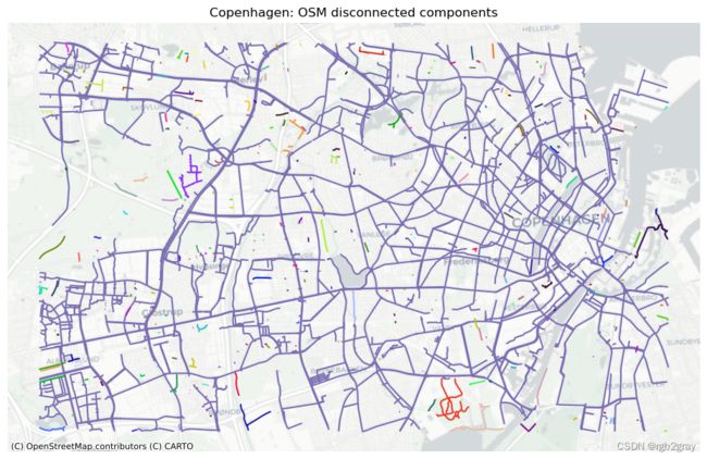
首先，在“return_components”的帮助下，获得网络的所有（断开连接的）组件的列表。 打印组件总数，并以不同颜色绘制所有组件以进行视觉分析。 接下来，绘制组件大小分布（组件按其包含的网络长度排序），然后绘制最大连接组件的图。

解释

与之前的许多分析步骤一样，该领域的知识对于正确解释成分分析至关重要。 鉴于数据准确地代表了实际的基础设施，较大的组件表示连贯的网络部分，而较小的组件表示分散的基础设施（例如，沿着街道的一条自行车道，不连接到任何其他自行车基础设施）。 大量彼此邻近的断开组件表明数字化错误或丢失数据。

4.1 断开的组件

osm_components = eval_func.return_components(osm_graph_simplified)
print(
    f"The network in the study area has {len(osm_components)} disconnected components."
)

The network in the study area has 356 disconnected components.

# Plot disconnected components

set_renderer(renderer_map)

# set seed for colors
np.random.seed(42)

# generate enough random colors to plot all components
randcols = np.random.rand(len(osm_components), 3)
randcols[0, :] = col_to_rgb(pdict['osm_base'])

fig, ax = plt.subplots(1, 1, figsize=pdict["fsmap"])

ax.set_title(f"{area_name}: OSM disconnected components")

ax.set_axis_off()

for j, c in enumerate(osm_components):
    if len(c.edges) > 0:
        edges = ox.graph_to_gdfs(c, nodes=False)
        edges.plot(ax=ax, color=randcols[j])

cx.add_basemap(ax=ax, crs=study_crs, source=cx_tile_2)

plot_func.save_fig(fig, osm_results_static_maps_fp + "all_components_osm")

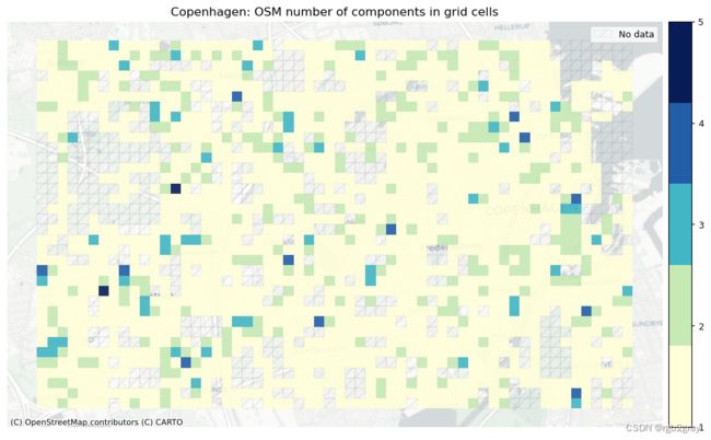
4.2 每个网格单元的组件

# Assign component ids to grid

grid = eval_func.assign_component_id_to_grid(
    osm_edges_simplified,
    osm_edges_simp_joined,
    osm_components,
    grid,
    prefix="osm",
    edge_id_col="edge_id",
)

fill_na_dict = {"component_ids_osm": ""}
grid.fillna(value=fill_na_dict, inplace=True)

grid["component_count_osm"] = grid.component_ids_osm.apply(lambda x: len(x))

# Plot number of components per grid cell

set_renderer(renderer_map)

fig, ax = plt.subplots(1, 1, figsize=pdict["fsmap"])

ncolors = grid["component_count_osm"].max()

from mpl_toolkits.axes_grid1 import make_axes_locatable
divider = make_axes_locatable(ax)
cax = divider.append_axes("right", size="3.5%", pad="1%")

mycm = cm.get_cmap(pdict["seq"], ncolors) 
grid[grid.component_count_osm>0].plot(
    cax=cax,
    ax=ax,
    column="component_count_osm",
    legend=True,
    legend_kwds={'ticks': list(range(1, ncolors+1))},
    cmap=mycm,
    alpha=pdict["alpha_grid"],
)

# add no data patches
grid[grid["count_osm_edges"].isnull()].plot(
    cax=cax,
    ax=ax,
    facecolor=pdict["nodata_face"],
    edgecolor=pdict["nodata_edge"],
    linewidth= pdict["line_nodata"],
    hatch=pdict["nodata_hatch"],
    alpha=pdict["alpha_nodata"],
)

ax.legend(handles=[nodata_patch], loc="upper right")

cx.add_basemap(ax=ax, crs=study_crs, source=cx_tile_2)
ax.set_title(area_name + ": OSM number of components in grid cells")
ax.set_axis_off()

plot_func.save_fig(fig, osm_results_static_maps_fp + f"number_of_components_in_grid_cells_osm")

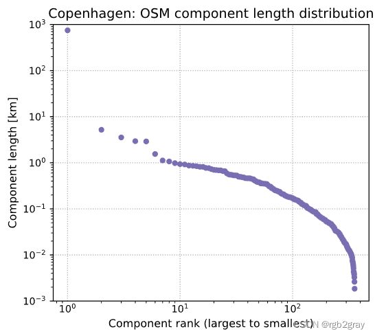
4.3 组件长度分布

所有网络组件长度的分布可以在所谓的 Zipf 图 中可视化，该图按等级对每个组件的长度进行排序，在左侧显示最大组件的长度，然后是第二大组件的长度，依此类推，直到 右侧最小组件的长度。 当 Zipf 图遵循 双对数比例 中的直线时，这意味着找到小的不连续组件的机会比传统分布的预期要高得多 (Clauset et al., 2009)。 这可能意味着网络没有合并，只有分段或随机添加 (Szell et al., 2022)，或者数据本身存在许多间隙和拓扑错误，导致小的断开组件。

但是，也可能发生最大的连通分量（图中最左边的标记，等级为 $10^0$）是明显的异常值，而图的其余部分则遵循不同的形状。 这可能意味着在基础设施层面，大部分基础设施已连接到一个大型组件，并且数据反映了这一点 - 即数据在很大程度上没有受到间隙和缺失链接的影响。

自行车网络也可能介于两者之间，有几个大型组件作为异常值。

# Zipf plot of component lengths

set_renderer(renderer_plot)

components_length = {}
for i, c in enumerate(osm_components):
    c_length = 0
    for (u, v, l) in c.edges(data="length"):
        c_length += l
    components_length[i] = c_length

components_df = pd.DataFrame.from_dict(components_length, orient="index")
components_df.rename(columns={0: "component_length"}, inplace=True)

fig = plt.figure(figsize=pdict["fsbar_small"])
axes = fig.add_axes([0, 0, 1, 1])

axes.set_axisbelow(True)
axes.grid(True,which="major",ls="dotted")
yvals = sorted(list(components_df["component_length"] / 1000), reverse = True)
axes.scatter(
    x=[i+1 for i in range(len(components_df))],
    y=yvals,
    s=18,
    color=pdict["osm_base"],
)
axes.set_ylim(ymin=10**math.floor(math.log10(min(yvals))), ymax=10**math.ceil(math.log10(max(yvals))))
axes.set_xscale("log")
axes.set_yscale("log")

axes.set_ylabel("Component length [km]")
axes.set_xlabel("Component rank (largest to smallest)")
axes.set_title(area_name+": OSM component length distribution")

plot_func.save_fig(fig, osm_results_plots_fp + "component_length_distribution_osm")

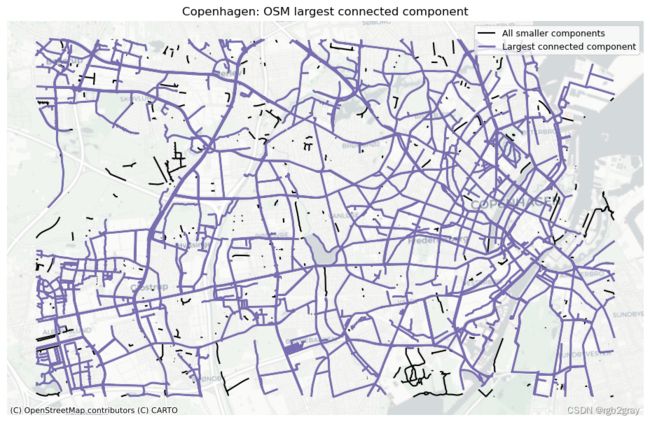
4.4 最大连通分量

largest_cc = max(osm_components, key=len)

largest_cc_length = 0

for (u, v, l) in largest_cc.edges(data="length"):

    largest_cc_length += l

largest_cc_pct = largest_cc_length / components_df["component_length"].sum() * 100

print(
    f"The largest connected component contains {largest_cc_pct:.2f}% of the network length."
)

# Get edges in largest cc
lcc_edges = ox.graph_to_gdfs(
    G=largest_cc, nodes=False, edges=True, node_geometry=False, fill_edge_geometry=False
)

# Export to GPKG
lcc_edges[["edge_id", "geometry"]].to_file(
    osm_results_data_fp + "largest_connected_component.gpkg"
)

The largest connected component contains 91.47% of the network length.

# Plot of largest connected component

set_renderer(renderer_map)
fig, ax = plt.subplots(1, 1, figsize=pdict["fsmap"])
osm_edges_simplified.plot(ax=ax, color = pdict["base"], linewidth = 1.5, label = "All smaller components")
lcc_edges.plot(ax=ax, color=pdict["osm_base"], linewidth = 2, label = "Largest connected component")
grid.plot(ax=ax,alpha=0)
ax.set_axis_off()
ax.set_title(area_name + ": OSM largest connected component")
ax.legend()

cx.add_basemap(ax=ax, crs=study_crs, source=cx_tile_2)

plot_func.save_fig(fig, osm_results_static_maps_fp + f"largest_conn_comp_osm")

# Save plot without basemap for potential report titlepage

set_renderer(renderer_map)
fig, ax = plt.subplots(1, 1, figsize=pdict["fsmap"])
osm_edges_simplified.plot(ax=ax, color = pdict["base"], linewidth = 1.5, label = "Disconnected components")
lcc_edges.plot(ax=ax, color=pdict["osm_base"], linewidth = 2, label = "Largest connected component")
ax.set_axis_off()

plot_func.save_fig(fig, osm_results_static_maps_fp + f"titleimage",plot_res="high")
plt.close()

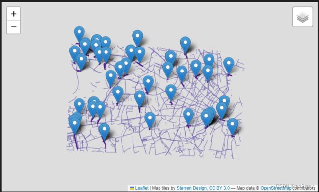
4.5 缺少链接

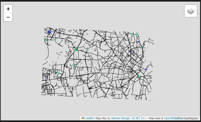
在组件之间潜在缺失链接的图中，将绘制与另一个组件上的边的指定距离内的所有边。 断开的边缘之间的间隙用标记突出显示。 因此，该地图突出显示了边缘，尽管这些边缘彼此非常接近，但它们是断开连接的，因此不可能在边缘之间的自行车基础设施上骑自行车。

User configuration

在分析组件之间潜在的缺失链接时，用户必须定义两个组件之间的距离被认为足够低以至于怀疑数字化错误的阈值。

# DEFINE MAX BUFFER DISTANCE BETWEEN COMPONENTS CONSIDERED A GAP/MISSING LINK
component_min_distance = 10

assert isinstance(component_min_distance, int) or isinstance(
    component_min_distance, float
), print("Setting must be integer or float value!")

print(f"Running analysis with component distance threshold of {component_min_distance} meters.")

Running analysis with component distance threshold of 10 meters.

component_gaps = eval_func.find_adjacent_components(
    components=osm_components,
    buffer_dist=component_min_distance,
    crs=study_crs,
    edge_id="edge_id",
)
component_gaps_gdf = gpd.GeoDataFrame.from_dict(
    component_gaps, orient="index", geometry="geometry", crs=study_crs
)

edge_ids = set(
    component_gaps_gdf["edge_id" + "_left"].to_list()
    + component_gaps_gdf["edge_id" + "_right"].to_list()
)

edge_ids = [int(i) for i in edge_ids]
edges_with_gaps = osm_edges_simplified.loc[osm_edges_simplified.edge_id.isin(edge_ids)]

# Save to csv
pd.DataFrame(edge_ids, columns=["edge_id"]).to_csv(
    osm_results_data_fp + f"component_gaps_edges_{component_min_distance}.csv",
    index=False,
)

# Export gaps to GPKG
component_gaps_gdf.to_file(
    osm_results_data_fp + f"component_gaps_centroids_{component_min_distance}.gpkg"
)

# Interactive plot of adjacent, potentially disconnected components

if len(component_gaps) > 0:

    simplified_edges_folium = plot_func.make_edgefeaturegroup(
        gdf=osm_edges_simplified,
        mycolor=pdict["osm_base"],
        myweight=pdict["line_base"],
        nametag="All edges",
        show_edges=True,
    )

    component_issues_edges_folium = plot_func.make_edgefeaturegroup(
        gdf=edges_with_gaps,
        mycolor=pdict["osm_emp"],
        myweight=pdict["line_emp"],
        nametag="Adjacent disconnected edges",
        show_edges=True,
    )

    component_issues_gaps_folium = plot_func.make_markerfeaturegroup(
        gdf=component_gaps_gdf, nametag="Component gaps", show_markers=True
    )

    m = plot_func.make_foliumplot(
        feature_groups=[
            simplified_edges_folium,
            component_issues_edges_folium,
            component_issues_gaps_folium,
        ],
        layers_dict=folium_layers,
        center_gdf=osm_nodes_simplified,
        center_crs=osm_nodes_simplified.crs,
    )

    bounds = plot_func.compute_folium_bounds(osm_nodes_simplified)
    m.fit_bounds(bounds)

    m.save(osm_results_inter_maps_fp + f"component_gaps_{component_min_distance}_osm.html")

    display(m)

if len(component_gaps) > 0:
    print("Interactive map saved at " + osm_results_inter_maps_fp.lstrip("../") + f"component_gaps_{component_min_distance}_osm.html")
else:
    print("There are no component gaps to plot.")

Interactive map saved at results/OSM/cph_geodk/maps_interactive/component_gaps_10_osm.html

4.6 组件连接

在这里，我们可视化每个单元格可以到达的单元格数量之间的差异。 这是对网络连接性的粗略测量，但具有计算成本低的优点，因此能够快速突出网络连接性的明显差异。

osm_components_cell_count = eval_func.count_component_cell_reach(
    components_df, grid, "component_ids_osm"
)
grid["cells_reached_osm"] = grid["component_ids_osm"].apply(
    lambda x: eval_func.count_cells_reached(x, osm_components_cell_count)
    if x != ""
    else 0
)

grid["cells_reached_osm_pct"] = grid.apply(
    lambda x: np.round((x.cells_reached_osm / len(grid)) * 100, 2), axis=1
)

grid.loc[grid["cells_reached_osm_pct"] == 0, "cells_reached_osm_pct"] = np.NAN

# Plot percent of cells reachable

set_renderer(renderer_map)
fig, ax = plt.subplots(1, 1, figsize=pdict["fsmap"])

# norm for color bars
cbnorm_reach = colors.Normalize(vmin=0, vmax=100)

from mpl_toolkits.axes_grid1 import make_axes_locatable
divider = make_axes_locatable(ax)
cax = divider.append_axes("right", size="3.5%", pad="1%")

grid[grid.cells_reached_osm_pct > 0].plot(
    cax=cax,
    ax=ax,
    column="cells_reached_osm_pct",
    legend=True,
    cmap=pdict["seq"],
    norm=cbnorm_reach,
    alpha=pdict["alpha_grid"],
)

osm_edges_simplified.plot(ax=ax, color=pdict["osm_emp"], linewidth=1)

# add no data patches
grid[grid["count_osm_edges"].isnull()].plot(
    cax=cax,
    ax=ax,
    facecolor=pdict["nodata_face"],
    edgecolor=pdict["nodata_edge"],
    linewidth= pdict["line_nodata"],
    hatch=pdict["nodata_hatch"],
    alpha=pdict["alpha_nodata"],
)

ax.legend(handles=[nodata_patch], loc="upper right")

cx.add_basemap(ax=ax, crs=study_crs, source=cx_tile_2)
ax.set_title(area_name+": OSM percent of cells reachable")
ax.set_axis_off()

plot_func.save_fig(fig, osm_results_static_maps_fp + "percent_cells_reachable_grid_osm")

components_results = {}
components_results["component_count"] = len(osm_components)
components_results["largest_cc_pct_size"] = largest_cc_pct
components_results["largest_cc_length"] = largest_cc_length
components_results["count_component_gaps"] = len(component_gaps)

5.概括

# Print out table summary of results

summarize_results = {**density_results, **components_results}

summarize_results["count_dangling_nodes"] = len(dangling_nodes)
summarize_results["count_intersection_issues"] = count_intersection_issues
summarize_results["count_overshoots"] = len(overshoots)
summarize_results["count_undershoots"] = len(undershoot_nodes)
summarize_results["count_incompatible_tags"] = sum(
    len(lst) for lst in incompatible_tags_results.values()
)

# Add total node count and total infrastructure length
summarize_results["total_nodes"] = len(osm_nodes_simplified)
summarize_results["total_length"] = osm_edges_simplified.infrastructure_length.sum() / 1000

summarize_results_df = pd.DataFrame.from_dict(summarize_results, orient="index")

summarize_results_df.rename({0: " "}, axis=1, inplace=True)

# Convert length to km
summarize_results_df.loc["largest_cc_length"] = (
    summarize_results_df.loc["largest_cc_length"] / 1000
)

summarize_results_df = summarize_results_df.reindex([
    'total_length',
    'protected_density_m_sqkm',
    'unprotected_density_m_sqkm',
    'mixed_density_m_sqkm',
    'edge_density_m_sqkm',
    'total_nodes',
    'count_dangling_nodes',
    'node_density_count_sqkm',
    'dangling_node_density_count_sqkm',
    'count_incompatible_tags',
    'count_overshoots',
    'count_undershoots',
    'count_intersection_issues',
    'component_count',
    'largest_cc_length',
    'largest_cc_pct_size', 
    'count_component_gaps'
     ])

rename_metrics = {
    "total_length": "Total infrastructure length (km)",
    "total_nodes": "Nodes",
    "edge_density_m_sqkm": "Bicycle infrastructure density (m/km2)",
    "node_density_count_sqkm": "Nodes per km2",
    "dangling_node_density_count_sqkm": "Dangling nodes per km2",
    "protected_density_m_sqkm": "Protected bicycle infrastructure density (m/km2)",
    "unprotected_density_m_sqkm": "Unprotected bicycle infrastructure density (m/km2)",
    "mixed_density_m_sqkm": "Mixed protection bicycle infrastructure density (m/km2)",
    "component_count": "Components",
    "largest_cc_pct_size": "Largest component's share of network length",
    "largest_cc_length": "Length of largest component (km)",
    "count_component_gaps": "Component gaps",
    "count_dangling_nodes": "Dangling nodes",
    "count_intersection_issues": "Missing intersection nodes",
    "count_overshoots": "Overshoots",
    "count_undershoots": "Undershoots",
    "count_incompatible_tags": "Incompatible tag combinations",
}

summarize_results_df.rename(rename_metrics, inplace=True)
summarize_results_df.style.pipe(format_osm_style)

Intrinsic Quality Metrics - OSM data

Total infrastructure length (km)	1,056
Protected bicycle infrastructure density (m/km2)	5,342
Unprotected bicycle infrastructure density (m/km2)	427
Mixed protection bicycle infrastructure density (m/km2)	55
Bicycle infrastructure density (m/km2)	5,825
Nodes	5,016
Dangling nodes	1,828
Nodes per km2	28
Dangling nodes per km2	10
Incompatible tag combinations	2
Overshoots	8
Undershoots	18
Missing intersection nodes	0
Components	356
Length of largest component (km)	747
Largest component's share of network length	91%
Component gaps	78

6.保存结果

all_results = {}

all_results["existing_tags"] = existing_tags_results
all_results["incompatible_tags_results"] = incompatible_tags_results
all_results["incompatible_tags_count"] = sum(
    len(lst) for lst in incompatible_tags_results.values()
)
all_results["network_density"] = density_results
all_results["count_intersection_issues"] = count_intersection_issues
all_results["count_overshoots"] = len(overshoots)
all_results["count_undershoots"] = len(undershoot_nodes)
all_results["dangling_node_count"] = len(dangling_nodes)
all_results["simplification_outcome"] = simplification_results
all_results["component_analysis"] = components_results

with open(osm_intrinsic_fp, "w") as outfile:
    json.dump(all_results, outfile)


# Save summary dataframe
summarize_results_df.to_csv(
    osm_results_data_fp + "intrinsic_summary_results.csv", index=True
)

# Save grid with results
with open(osm_intrinsic_grid_fp, "wb") as f:
    pickle.dump(grid, f)

---

from time import strftime
print("Time of analysis: " + strftime("%a, %d %b %Y %H:%M:%S"))