水质预测模型

水质预测模型构建

1.水质数据介绍

1.1数据介绍

本文将水质分为可以用和不可饮用两种，以区分其水质好坏。水质数据来自于开源竞赛网络，具体包括pH value（pH值）、Hardness（硬度）、Solids（总溶解固体-TDS）、Chloramines（氯胺）、Conductivity（电导率）、Organic_carbon（有机碳）、Trihalomethanes（三卤甲烷类）、Turbidity（浊度）、Potability（可饮用性），以下是数据概念介绍。

• 1.pH value（pH值）
• PH是评估水的酸碱平衡的一个重要参数。它也是水状态的酸性或碱性条件的指示器。世界卫生组织建议pH值的最大允许限值为6.5至8.5。目前的调查范围为6.52-6.83，属于世界卫生组织标准范围。
• 2.Hardness（硬度）
• 硬度主要由钙盐和镁盐引起。这些盐是从水通过的地质沉积物中溶解出来的。水与产生硬度的材料接触的时间长度有助于确定原水中的硬度。硬度最初被定义为由钙和镁引起的水沉淀肥皂的能力。
• 3.Solids（总溶解固体-TDS）
• 水能够溶解各种无机和一些有机矿物或盐，如钾、钙、钠、碳酸氢盐、氯化物、镁、硫酸盐等。这些矿物在水的外观上会产生不想要的味道和稀释的颜色。这是用水的重要参数。TDS值高的水表明水具有高度矿化。TDS的理想限值为500mg/l，最大限值为1000mg/l，用于饮用。
• 4.Chloramines（氯胺）
• 氯和氯胺是公共供水系统中使用的主要消毒剂。氯胺最常见的形成是在氯中加入氨来处理饮用水。氯含量高达每升4毫克（mg/L或百万分之四（ppm））被认为是安全的饮用水中。
• 5.Sulfate（硫酸盐）
• 硫酸盐是天然存在的物质，存在于矿物、土壤和岩石中。它们存在于环境空气、地下水、植物和食物中。硫酸盐的主要商业用途是在化学工业中。海水中的硫酸盐浓度约为2700毫克/升（mg/L）。在大多数淡水供应中，它的浓度在3至30mg/L之间，尽管在一些地理位置发现的浓度要高得多（1000mg/L）。
• 6.Conductivity（电导率）
• 纯水不是电流的良好导体，而是一种良好的绝缘体。离子浓度的增加增强了水的导电性。通常，水中溶解固体的量决定了电导率。电导率（EC）实际上是测量溶液的离子过程，使其能够传输电流。根据世界卫生组织标准，EC值不应超过400μS/cm。
• 7.Organic_carbon（有机碳）
• 源水中的总有机碳（TOC）来自腐烂的天然有机物（NOM）和合成来源。TOC是衡量纯水中有机化合物中碳总量的指标。根据美国环保局的规定，经处理/饮用水中的总有机碳含量<2mg/L，用于处理的水源水中的总含量<4mg/L。
• 8.Trihalomethanes（三卤甲烷类）
• THM是一种化学物质，可能存在于经过氯处理的水中。饮用水中THM的浓度根据水中有机物质的水平、处理水所需的氯的量以及被处理水的温度而变化。高达80ppm的THM在饮用水中被认为是安全的。
• 9.Turbidity（浊度）
• 水的浊度取决于悬浮状态下存在的固体物质的数量。这是对水的发光财产的测量，该测试用于指示与胶体物质有关的废物排放质量。WondoGenet校园的平均浊度值（0.98NTU）低于世界卫生组织建议的5.00NTU。
• 10.Potability（可饮用性）
• 表示水对人类消费是否安全，其中1表示可饮用，0表示不可饮用。

import numpy as np
import pandas as pd
import seaborn as sns
import matplotlib.pyplot as plt
%matplotlib inline
import plotly.express as px
import warnings
warnings.filterwarnings('ignore')

# It is always consider as a good practice to make a copy of original dataset.

main_df = pd.read_csv("/kaggle/input/water-potability/water_potability.csv")
df = main_df.copy()

# 前5行数据
# Getting top 5 row of the dataset
df.head()

	ph	Hardness	Solids	Chloramines	Sulfate	Conductivity	Organic_carbon	Trihalomethanes	Turbidity	Potability
0	NaN	204.890455	20791.318981	7.300212	368.516441	564.308654	10.379783	86.990970	2.963135	0
1	3.716080	129.422921	18630.057858	6.635246	NaN	592.885359	15.180013	56.329076	4.500656	0
2	8.099124	224.236259	19909.541732	9.275884	NaN	418.606213	16.868637	66.420093	3.055934	0
3	8.316766	214.373394	22018.417441	8.059332	356.886136	363.266516	18.436524	100.341674	4.628771	0
4	9.092223	181.101509	17978.986339	6.546600	310.135738	398.410813	11.558279	31.997993	4.075075	0

Following are the list of algorithms that are used in this notebook.

Algorithm
Logistic Regression
Decision Tree
Random Forest
XGBoost
KNeighbours
SVM
AdaBoost

print(df.shape)

(3276, 10)

print(df.columns)

Index(['ph', 'Hardness', 'Solids', 'Chloramines', 'Sulfate', 'Conductivity',
       'Organic_carbon', 'Trihalomethanes', 'Turbidity', 'Potability'],
      dtype='object')

1.2描述性统计

• 各个数据的数量、平均值、标准差、最小最大值等如下表所示。

df.describe()

	ph	Hardness	Solids	Chloramines	Sulfate	Conductivity	Organic_carbon	Trihalomethanes	Turbidity	Potability
count	2785.000000	3276.000000	3276.000000	3276.000000	2495.000000	3276.000000	3276.000000	3114.000000	3276.000000	3276.000000
mean	7.080795	196.369496	22014.092526	7.122277	333.775777	426.205111	14.284970	66.396293	3.966786	0.390110
std	1.594320	32.879761	8768.570828	1.583085	41.416840	80.824064	3.308162	16.175008	0.780382	0.487849
min	0.000000	47.432000	320.942611	0.352000	129.000000	181.483754	2.200000	0.738000	1.450000	0.000000
25%	6.093092	176.850538	15666.690297	6.127421	307.699498	365.734414	12.065801	55.844536	3.439711	0.000000
50%	7.036752	196.967627	20927.833607	7.130299	333.073546	421.884968	14.218338	66.622485	3.955028	0.000000
75%	8.062066	216.667456	27332.762127	8.114887	359.950170	481.792304	16.557652	77.337473	4.500320	1.000000
max	14.000000	323.124000	61227.196008	13.127000	481.030642	753.342620	28.300000	124.000000	6.739000	1.000000

df.info()

RangeIndex: 3276 entries, 0 to 3275
Data columns (total 10 columns):
 #   Column           Non-Null Count  Dtype  
---  ------           --------------  -----  
 0   ph               2785 non-null   float64
 1   Hardness         3276 non-null   float64
 2   Solids           3276 non-null   float64
 3   Chloramines      3276 non-null   float64
 4   Sulfate          2495 non-null   float64
 5   Conductivity     3276 non-null   float64
 6   Organic_carbon   3276 non-null   float64
 7   Trihalomethanes  3114 non-null   float64
 8   Turbidity        3276 non-null   float64
 9   Potability       3276 non-null   int64  
dtypes: float64(9), int64(1)
memory usage: 256.1 KB

#数量

print(df.nunique())

ph                 2785
Hardness           3276
Solids             3276
Chloramines        3276
Sulfate            2495
Conductivity       3276
Organic_carbon     3276
Trihalomethanes    3114
Turbidity          3276
Potability            2
dtype: int64

# 唯一值数量
print(df.isnull().sum())

ph                 491
Hardness             0
Solids               0
Chloramines          0
Sulfate            781
Conductivity         0
Organic_carbon       0
Trihalomethanes    162
Turbidity            0
Potability           0
dtype: int64

#定义各指标数据类型

df.dtypes

ph                 float64
Hardness           float64
Solids             float64
Chloramines        float64
Sulfate            float64
Conductivity       float64
Organic_carbon     float64
Trihalomethanes    float64
Turbidity          float64
Potability           int64
dtype: object

sns.heatmap(df.isnull())

#各指标关联矩阵

plt.figure(figsize=(10, 8))
sns.heatmap(df.corr(), annot= True, cmap='coolwarm')

#拆解关联矩阵来更直观的查看指标间的关联性

# Unstacking the correlation matrix to see the values more clearly.
corr = df.corr()
c1 = corr.abs().unstack()
c1.sort_values(ascending = False)[12:24:2]

Hardness  Sulfate           0.106923
ph        Solids            0.089288
Hardness  ph                0.082096
Solids    Chloramines       0.070148
Hardness  Solids            0.046899
ph        Organic_carbon    0.043503
dtype: float64

#可饮用数据与不可饮用数据柱状图

ax = sns.countplot(x = "Potability",data= df, saturation=0.8)
plt.xticks(ticks=[0, 1], labels = ["Not Potable", "Potable"])
plt.show()






    



```python
#可饮数据与不可饮用数据

x = df.Potability.value_counts()
labels = [0,1]
print(x)

0    1998
1    1278
Name: Potability, dtype: int64

#PH值和可饮用性的小提琴图

sns.violinplot(x='Potability', y='ph', data=df, palette='rocket')

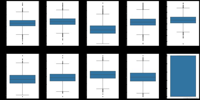
#用箱线图可视化数据并检查异常值

# Visualizing dataset and also checking for outliers 

fig, ax = plt.subplots(ncols = 5, nrows = 2, figsize = (20, 10))
index = 0
ax = ax.flatten()

for col, value in df.items():
    sns.boxplot(y=col, data=df, ax=ax[index])
    index += 1
plt.tight_layout(pad = 0.5, w_pad=0.7, h_pad=5.0)

#用柱状图可视化数据

plt.rcParams['figure.figsize'] = [20,10]
df.hist()
plt.show()

#根据可饮用性进行分类

sns.pairplot(df, hue="Potability")

#可饮用性（x轴）和密度（y轴）的关系

plt.rcParams['figure.figsize'] = [7,5]
sns.distplot(df['Potability'])

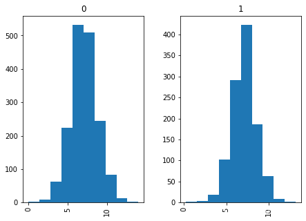
#PH值与可饮用性的关系

df.hist(column='ph', by='Potability')

array([,
       ], dtype=object)

#水质硬度与可饮用性的关系

df.hist(column='Hardness', by='Potability')

array([,
       ], dtype=object)

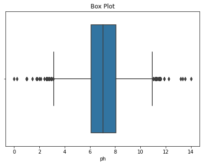
#各指标的独立箱线图

# Individual box plot for each feature
def Box(df):
    plt.title("Box Plot")
    sns.boxplot(df)
    plt.show()
Box(df['ph'])

#水质硬化不同程度的数量

sns.histplot(x = "Hardness", data=df)

#获取唯一值

df.nunique()

ph                 2785
Hardness           3276
Solids             3276
Chloramines        3276
Sulfate            2495
Conductivity       3276
Organic_carbon     3276
Trihalomethanes    3114
Turbidity          3276
Potability            2
dtype: int64

#对各指标的影响程度按降序排列

skew_val = df.skew().sort_values(ascending=False)
skew_val

Solids             0.621634
Potability         0.450784
Conductivity       0.264490
ph                 0.025630
Organic_carbon     0.025533
Turbidity         -0.007817
Chloramines       -0.012098
Sulfate           -0.035947
Hardness          -0.039342
Trihalomethanes   -0.083031
dtype: float64

• Using pandas skew function to check the correlation between the values.
• Values between 0.5 to -0.5 will be considered as the normal distribution else will be skewed depending upon the skewness value.

#各指标缺失数据的百分比

df.isnull().mean().plot.bar(figsize=(10,6)) 
plt.ylabel('Percentage of missing values') 
plt.xlabel('Features') 
plt.title('Missing Data in Percentages');

df['ph'] = df['ph'].fillna(df['ph'].mean())
df['Sulfate'] = df['Sulfate'].fillna(df['Sulfate'].mean())
df['Trihalomethanes'] = df['Trihalomethanes'].fillna(df['Trihalomethanes'].mean())

df.head()

	ph	Hardness	Solids	Chloramines	Sulfate	Conductivity	Organic_carbon	Trihalomethanes	Turbidity	Potability
0	7.080795	204.890455	20791.318981	7.300212	368.516441	564.308654	10.379783	86.990970	2.963135	0
1	3.716080	129.422921	18630.057858	6.635246	333.775777	592.885359	15.180013	56.329076	4.500656	0
2	8.099124	224.236259	19909.541732	9.275884	333.775777	418.606213	16.868637	66.420093	3.055934	0
3	8.316766	214.373394	22018.417441	8.059332	356.886136	363.266516	18.436524	100.341674	4.628771	0
4	9.092223	181.101509	17978.986339	6.546600	310.135738	398.410813	11.558279	31.997993	4.075075	0

#各数据的热力图

sns.heatmap(df.isnull())

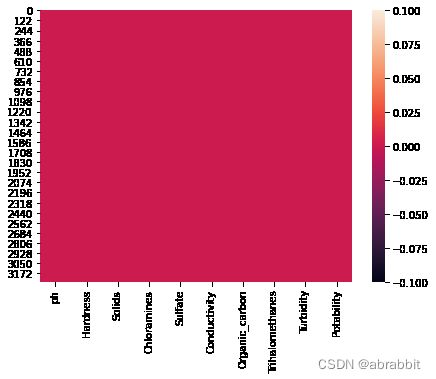
df.isnull().sum()

ph                 0
Hardness           0
Solids             0
Chloramines        0
Sulfate            0
Conductivity       0
Organic_carbon     0
Trihalomethanes    0
Turbidity          0
Potability         0
dtype: int64

X = df.drop('Potability', axis=1)
y = df['Potability']

X.shape, y.shape

((3276, 9), (3276,))

# import StandardScaler to perform scaling
from sklearn.preprocessing import StandardScaler 
scaler = StandardScaler()

X = scaler.fit_transform(X)
X

array([[-1.02733269e-14,  2.59194711e-01, -1.39470871e-01, ...,
        -1.18065057e+00,  1.30614943e+00, -1.28629758e+00],
       [-2.28933938e+00, -2.03641367e+00, -3.85986650e-01, ...,
         2.70597240e-01, -6.38479983e-01,  6.84217891e-01],
       [ 6.92867789e-01,  8.47664833e-01, -2.40047337e-01, ...,
         7.81116857e-01,  1.50940884e-03, -1.16736546e+00],
       ...,
       [ 1.59125368e+00, -6.26829230e-01,  1.27080989e+00, ...,
        -9.81329234e-01,  2.18748247e-01, -8.56006782e-01],
       [-1.32951593e+00,  1.04135450e+00, -1.14405809e+00, ...,
        -9.42063817e-01,  7.03468419e-01,  9.50797383e-01],
       [ 5.40150905e-01, -3.85462310e-02, -5.25811937e-01, ...,
         5.60940070e-01,  7.80223466e-01, -2.12445866e+00]])

# import train-test split 
from sklearn.model_selection import train_test_split

X_train, X_test, y_train, y_test = train_test_split(X, y, test_size=0.33, random_state=42)

2.水质模型构建

2.1逻辑回归模型构建

这几个水质模型构建效果分析（结合各模型图表、指标）

from sklearn.linear_model import LogisticRegression
from sklearn.metrics import confusion_matrix, accuracy_score, classification_report

# Creating model object
model_lg = LogisticRegression(max_iter=120,random_state=0, n_jobs=20)

# Training Model
model_lg.fit(X_train, y_train)

LogisticRegression(max_iter=120, n_jobs=20, random_state=0)

# Making Prediction
pred_lg = model_lg.predict(X_test)

# Calculating Accuracy Score
lg = accuracy_score(y_test, pred_lg)
print(lg)

0.6284658040665434

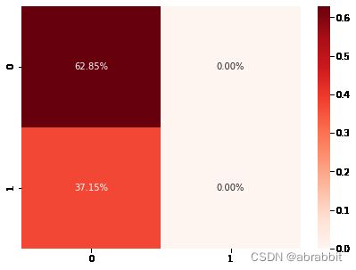
• 逻辑回归的预测精确度为0.6284658040665434

print(classification_report(y_test,pred_lg))

              precision    recall  f1-score   support

           0       0.63      1.00      0.77       680
           1       0.00      0.00      0.00       402

    accuracy                           0.63      1082
   macro avg       0.31      0.50      0.39      1082
weighted avg       0.39      0.63      0.49      1082

• 逻辑回归的召回率、f1分数如上图所示。

# confusion Maxtrix
cm1 = confusion_matrix(y_test, pred_lg)
sns.heatmap(cm1/np.sum(cm1), annot = True, fmt=  '0.2%', cmap = 'Reds')

2.2决策树模型构建

from sklearn.tree import DecisionTreeClassifier

# Creating model object
model_dt = DecisionTreeClassifier( max_depth=4, random_state=42)

# Training Model
model_dt.fit(X_train,y_train)

DecisionTreeClassifier(max_depth=4, random_state=42)

# Making Prediction
pred_dt = model_dt.predict(X_test)

# Calculating Accuracy Score
dt = accuracy_score(y_test, pred_dt)
print(dt)

0.6451016635859519

• 可见，决策树模型的精确度是0.6451016635859519

print(classification_report(y_test,pred_dt))

              precision    recall  f1-score   support

           0       0.66      0.90      0.76       680
           1       0.56      0.22      0.32       402

    accuracy                           0.65      1082
   macro avg       0.61      0.56      0.54      1082
weighted avg       0.62      0.65      0.60      1082

• 决策树模型的召回率、f1分数如上图所示。

# confusion Maxtrix
cm2 = confusion_matrix(y_test, pred_dt)
sns.heatmap(cm2/np.sum(cm2), annot = True, fmt=  '0.2%', cmap = 'Reds')

2.3随机森林模型构建

from sklearn.ensemble import RandomForestClassifier

# Creating model object
model_rf = RandomForestClassifier(n_estimators=300,min_samples_leaf=0.16, random_state=42)

# Training Model
model_rf.fit(X_train, y_train)

RandomForestClassifier(min_samples_leaf=0.16, n_estimators=300, random_state=42)

# Making Prediction
pred_rf = model_rf.predict(X_test)

# Calculating Accuracy Score
rf = accuracy_score(y_test, pred_rf)
print(rf)

0.6284658040665434

随机森林模型的准确度是0.6284658040665434

print(classification_report(y_test,pred_rf))

              precision    recall  f1-score   support

           0       0.63      1.00      0.77       680
           1       0.00      0.00      0.00       402

    accuracy                           0.63      1082
   macro avg       0.31      0.50      0.39      1082
weighted avg       0.39      0.63      0.49      1082

• 随机森林模型的召回率、f1分数如上图所示。

# confusion Maxtrix
cm3 = confusion_matrix(y_test, pred_rf)
sns.heatmap(cm3/np.sum(cm3), annot = True, fmt=  '0.2%', cmap = 'Reds')

2.4XGBoost模型构建

from xgboost import XGBClassifier

# Creating model object
model_xgb = XGBClassifier(max_depth= 8, n_estimators= 125, random_state= 0,  learning_rate= 0.03, n_jobs=5)

# Training Model
model_xgb.fit(X_train, y_train)

[01:40:53] WARNING: ../src/learner.cc:1095: Starting in XGBoost 1.3.0, the default evaluation metric used with the objective 'binary:logistic' was changed from 'error' to 'logloss'. Explicitly set eval_metric if you'd like to restore the old behavior.





XGBClassifier(base_score=0.5, booster='gbtree', colsample_bylevel=1,
              colsample_bynode=1, colsample_bytree=1, gamma=0, gpu_id=-1,
              importance_type='gain', interaction_constraints='',
              learning_rate=0.03, max_delta_step=0, max_depth=8,
              min_child_weight=1, missing=nan, monotone_constraints='()',
              n_estimators=125, n_jobs=5, num_parallel_tree=1, random_state=0,
              reg_alpha=0, reg_lambda=1, scale_pos_weight=1, subsample=1,
              tree_method='exact', validate_parameters=1, verbosity=None)

# Making Prediction
pred_xgb = model_xgb.predict(X_test)

# Calculating Accuracy Score
xgb = accuracy_score(y_test, pred_xgb)
print(xgb)

0.6709796672828097

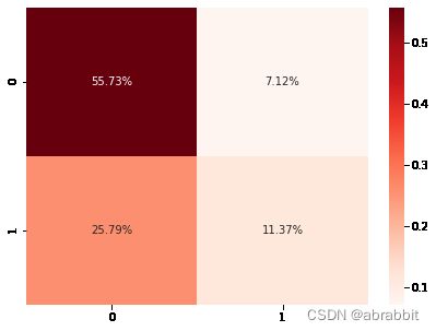
• XGBoost模型的准确度是0.6709796672828097

print(classification_report(y_test,pred_xgb))

              precision    recall  f1-score   support

           0       0.68      0.89      0.77       680
           1       0.61      0.31      0.41       402

    accuracy                           0.67      1082
   macro avg       0.65      0.60      0.59      1082
weighted avg       0.66      0.67      0.64      1082

• XGBoost模型的召回率、F1分数指标如上图所示。

# confusion Maxtrix
cm4 = confusion_matrix(y_test, pred_xgb)
sns.heatmap(cm4/np.sum(cm4), annot = True, fmt=  '0.2%', cmap = 'Reds')

2.5KNN模型构建

from sklearn.neighbors import KNeighborsClassifier

# Creating model object
model_kn = KNeighborsClassifier(n_neighbors=9, leaf_size=20)

# Training Model
model_kn.fit(X_train, y_train)

KNeighborsClassifier(leaf_size=20, n_neighbors=9)

# Making Prediction
pred_kn = model_kn.predict(X_test)

# Calculating Accuracy Score
kn = accuracy_score(y_test, pred_kn)
print(kn)

0.6534195933456562

• KNN模型的准确度是0.6534195933456562

print(classification_report(y_test,pred_kn))

              precision    recall  f1-score   support

           0       0.69      0.82      0.75       680
           1       0.55      0.37      0.44       402

    accuracy                           0.65      1082
   macro avg       0.62      0.60      0.59      1082
weighted avg       0.64      0.65      0.63      1082

• KNN模型的召回率、f1分数如上图所示。

# confusion Maxtrix
cm5 = confusion_matrix(y_test, pred_kn)
sns.heatmap(cm5/np.sum(cm5), annot = True, fmt=  '0.2%', cmap = 'Reds')

2.6支持向量机模型构建

from sklearn.svm import SVC, LinearSVC

model_svm = SVC(kernel='rbf', random_state = 42)

model_svm.fit(X_train, y_train)

SVC(random_state=42)

# Making Prediction
pred_svm = model_svm.predict(X_test)

# Calculating Accuracy Score
sv = accuracy_score(y_test, pred_svm)
print(sv)

0.6885397412199631

print(classification_report(y_test,pred_kn))

# confusion Maxtrix
cm6 = confusion_matrix(y_test, pred_svm)
sns.heatmap(cm6/np.sum(cm6), annot = True, fmt=  '0.2%', cmap = 'Reds')

## Using AdaBoost Classifier

from sklearn.ensemble import AdaBoostClassifier

model_ada = AdaBoostClassifier(learning_rate= 0.002,n_estimators= 205,random_state=42)

model_ada.fit(X_train, y_train)

AdaBoostClassifier(learning_rate=0.002, n_estimators=205, random_state=42)

# Making Prediction
pred_ada = model_ada.predict(X_test)

# Calculating Accuracy Score
ada = accuracy_score(y_test, pred_ada)
print(ada)

0.634011090573013

• 可见，SVM模型准确率是0.634011090573013

print(classification_report(y_test,pred_ada))

              precision    recall  f1-score   support

           0       0.63      0.99      0.77       680
           1       0.62      0.04      0.07       402

    accuracy                           0.63      1082
   macro avg       0.62      0.51      0.42      1082
weighted avg       0.63      0.63      0.51      1082

• SVM模型的召回率、F1分数如上图所示。

# confusion Maxtrix
cm7 = confusion_matrix(y_test, pred_ada)
sns.heatmap(cm7/np.sum(cm7), annot = True, fmt=  '0.2%', cmap = 'Reds')

3.各模型效果比较

models = pd.DataFrame({
    'Model':['Logistic Regression', 'Decision Tree', 'Random Forest', 'XGBoost', 'KNeighbours', 'SVM', 'AdaBoost'],
    'Accuracy_score' :[lg, dt, rf, xgb, kn, sv, ada]
})
models
sns.barplot(x='Accuracy_score', y='Model', data=models)

models.sort_values(by='Accuracy_score', ascending=False)

	Model	Accuracy_score
5	SVM	0.688540
3	XGBoost	0.670980
4	KNeighbours	0.653420
1	Decision Tree	0.645102
6	AdaBoost	0.634011
0	Logistic Regression	0.628466
2	Random Forest	0.628466

比较了各个模型的预测精度后发现，SVM模型有着更高的精准度。