李沐之神经网络基础
目录
1.模型构造
1.1层和块
1.2自定义块
1.3顺序块
1.4在前向传播函数中执行代码
2.参数管理
2.1参数访问
2.2参数初始化
3.自定义层
3.1不带参数的层
3.2带参数的层
4.读写文件
4.1加载和保存张量
4.2加载和保存模型参数
1.模型构造
1.1层和块
import torch
from torch import nn
from torch.nn import functional as F
#定义了一些没有包括参数的函数

net = nn.Sequential(nn.Linear(20, 256), nn.ReLU(), nn.Linear(256, 10))
#构造的单层神经网络,线性层,激活层,线性层

X = torch.rand(2, 20)
#生成一个随机的input,torch.rand是用于生成均匀随机分布张量的函数,从区间[0,1)的均匀分布中
#随机抽取一个随机数生成一个张量,其中2是批量大小,20是输入的维度。
net(X)

"""输出结果:
tensor([[ 0.0343,  0.0264,  0.2505, -0.0243,  0.0945,  0.0012, -0.0141,  0.0666,
         -0.0547, -0.0667],
        [ 0.0772, -0.0274,  0.2638, -0.0191,  0.0394, -0.0324,  0.0102,  0.0707,
         -0.1481, -0.1031]], grad_fn=)"""
1.2自定义块
#任何一个层和任何一个神经网络应该都是muodule的一个子类
class MLP(nn.Module):
#定义了一个MLP类继承nn.Module:
    def __init__(self):
    # 调用MLP的父类Module的构造函数来执行必要的初始化。
    # 这样,在类实例化时也可以指定其他函数参数,例如模型参数params(稍后将介绍)
    #在init函数里面定义了需要的函数和参数,在运行类对象的时候可以自动传递参数给属性,
    #和运行方法
        super().__init__(self):
        #调用父类nn.Module成员方法,把所需要的内部参数给全部设好
        self.hidden=nn.Linear(20,256)
        self.out=nn.Linear(256,10)
        #定义两个全连接层
    #__init__函数包括了网络里面需要的全部的层


    # 定义模型的前向传播,即如何根据输入X返回所需的模型输出
    def forward(self,x):
        return self.out(F.relu(self.hidden()))
        #F里面实现了很多的常用的和函数,注意,这里我们使用ReLU的函数版本,
        #其在nn.functional模块中定义。

#实例化多层感知机的层,然后在每次调用前向传播函数时调用这些层。注意一些关键细节: 首先,
#我们定制的__init__函数通过super().__init__() 调用父类的__init__函数, 省去了重复编写
#模版代码的痛苦。 然后,我们实例化两个全连接层, 分别为self.hidden和self.out。 注意,
#除非我们实现一个新的运算符, 否则我们不必担心反向传播函数或参数初始化, 系统将自动生成这些。

net=MLP()
net(X)
#这里可以直接调用net(x)而不是net.forward(x)的原因是nn.Module() 中包含了 __call__ 函数
"""输出结果:
tensor([[ 0.0669,  0.2202, -0.0912, -0.0064,  0.1474, -0.0577, -0.3006,  0.1256,
         -0.0280,  0.4040],
        [ 0.0545,  0.2591, -0.0297,  0.1141,  0.1887,  0.0094, -0.2686,  0.0732,
         -0.0135,  0.3865]], grad_fn=)"""
块的一个主要优点是它的多功能性。 我们可以子类化块以创建层(如全连接层的类)、 整个模型(如上面的MLP类)或具有中等复杂度的各种组件。 我们在接下来的章节中充分利用了这种多功能性, 比如在处理卷积神经网络时。
1.3顺序块
class MySequential(nn.Module):
    def __init__(self,*args):
    #*表示接受不定长参数传递
        super().__init__()
        for idx,module in enumerate(args):
        #这里,module是Module子类的一个实例。我们把它保存在'Module'类的成员,
        #变量_modules中。_module的类型是OrderedDict

        #enumerate()函数用于将一个可遍历的数据对象(如列表、元组或字符串)组合为一个索引
        #序列,同时列出数据和数据下标(把序号和内容打包在一起),一般用在 for 循环当中。
        #idx是序号,module是内容(也就是层)
        self._modules[str(idx)]=module
        #enumerate返回的是一个枚举对象,把索引转换成字符串使之可以被顺序访问
        #写入字典中

    def forward(self,X):
        # OrderedDict保证了按照成员添加的顺序遍历它们
        for block in self._modiles.values():
            X=block(X)
        return X

net=MySequential(nn.Linear(20,256),nn.ReLU(),nn.Linear(256,10))
net(X)
"""结果输出:
tensor([[ 2.2759e-01, -4.7003e-02,  4.2846e-01, -1.2546e-01,  1.5296e-01,
          1.8972e-01,  9.7048e-02,  4.5479e-04, -3.7986e-02,  6.4842e-02],
        [ 2.7825e-01, -9.7517e-02,  4.8541e-01, -2.4519e-01, -8.4580e-02,
          2.8538e-01,  3.6861e-02,  2.9411e-02, -1.0612e-01,  1.2620e-01]],
       grad_fn=)
"""
__init__函数将每个模块逐个添加到有序字典_modules中。_modules的主要优点是: 在模块的参数初始化过程中, 系统知道在_modules字典中查找需要初始化参数的子块。当MySequential的前向传播函数被调用时, 每个添加的块都按照它们被添加的顺序执行。 现在可以使用我们的MySequential类重新实现多层感知机。
1.4在前向传播函数中执行代码

class FixedHiddenMLP(nn.Module):
    def __init__(self):
        super().__init__()
        # 不计算梯度的随机权重参数。因此其在训练期间保持不变
        self.rand_weight=torch.rand((20,20),requires_grad=False)
        #形状是20*20
        self.linear=nn.Linear(20,20)
        #nn.Linear其中第一个维度是batch_size,第二个维度是输入特征的数量。输出是
        #一个二维张量,其中第一个维度是batch_size,第二个维度是输出特征的数量。

        def forward(self,X):
            X=self.linear(X)
            #使用创建的常量参数以及relu和mm函数
            X=F.relu(torch.mm(X,self.rand_weight)+1)
            # 复用全连接层。这相当于两个全连接层共享参数
            X=self.linear(X)
            # 控制流
            while X.abs().sum()>1:
            #当绝对值求和大于1(l1范数)就一直除以2
                X/=2
            return X.sum
            #返回的是标量

net = FixedHiddenMLP()
net(X)
"""结果输出:
tensor(-0.2160, grad_fn=)"""


#混合搭配各种组合块的方法
class NestMLP(nn.Module):
    def __init__(self):
        super().__init__()
        self.net=nn.Sequential(nn.Linear(20,64),nn.ReLU(),nn.Linear(),nn.ReLU())
        self.linear=nn.Linear(32,16)

    def forward(self,X):
        return self.linear(self.net(X))

chimera=nn.Sequential(NestMLP(),nn.Linear(16,20),FixedHiddenMLP())
chimera(X)
"""结果输出:
tensor(0.2183, grad_fn=)
""" 
2.参数管理
2.1参数访问
#首先关注具有单隐藏层的多层感知机
import torch
from torch import nn
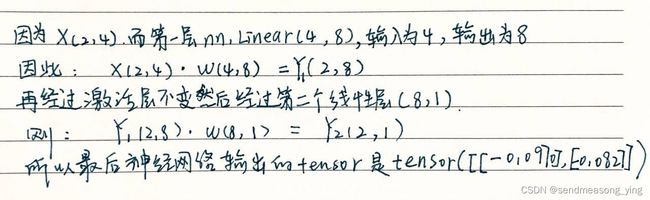
net=nn.Sequential(nn.Linear(4,8),nn.ReLU(),nn.Linear(8,1))
#nn.Linear(4,8)表示输入为4,输出为8
X=torch.rand(size=(2,4))
#X的形状是(2*4),表示有2个样本
net(X)
"""结果输出:
tensor([[-0.0619],
[-0.0489]], grad_fn=)"""
"""参数访问"""
print(net[2].state_dict())
#net[2]拿到的是最后一个线性层,权重是一个状态state,因为权重可以被改变
"""结果输出:
OrderedDict([('weight', tensor([[-0.0427, -0.2939, -0.1894, 0.0220, -0.1709, -0.1522, -0.0334, -0.2263]])),
('bias', tensor([0.0887]))])
"""
#8个权重,1个偏置.输出的结果告诉我们一些重要的事情: 首先,这个全连接层包含两个参数,
#分别是该层的权重和偏置。 两者都存储为单精度浮点数(float32)。 注意,参数名称允许唯
#一标识每个参数,即使在包含数百个层的网络中也是如此。
"""目标参数"""
print(type(net[2].bias))
print(net[2].bias)
print(net[2].bias.data)
"""结果输出:
Parameter containing:
tensor([-0.0291], requires_grad=True)
tensor([-0.0291])"""
#参数是复合的对象,包含值、梯度和额外信息。 这就是我们需要显式参数值的原因。 除了值之外,
#我们还可以访问每个参数的梯度。
net[2].weight.grad==None
"""结果输出:
True"""
#在上面这个网络中,由于我们还没有调用反向传播(没有计算loss,W,B没有更新,所以没有反向计算),
#所以参数的梯度处于初始状态。
"""一次性访问所有参数"""
#当我们需要对所有参数执行操作时,逐个访问它们可能会很麻烦。 当我们处理更复杂的块
#(例如,嵌套块)时,情况可能会变得特别复杂, 因为我们需要递归整个树来提取每个子块的参数。
#下面,我们将通过演示来比较访问第一个全连接层的参数和访问所有层。
print(*[(name,param.shape) for name,param in net[0].named_parameters()])
print(*[(name,param.shape) for name,param in net.named_parameters()])
"""结果输出:
('weight', torch.Size([8, 4])) ('bias', torch.Size([8]))
('0.weight', torch.Size([8, 4])) ('0.bias', torch.Size([8])) ('2.weight', torch.Size([1, 8]))
'2.bias', torch.Size([1]))"""
#理解一下为什么是[8,4]因为这是权重X要和权重进行矩阵乘法,而
#另一种访问网络参数的方式
net.state_dict()['2.bias'].data
"""结果输出:
tensor([-0.0291])"""
"""从嵌套块收集参数"""
def block1():
return nn.Sequential(nn.Linear(4,8),nn.ReLU(),nn.Linear(),nn.ReLU())
def block2():
net=nn.Sequential()
for i in range(4):
#在这里嵌套
net.add_module(f'block{i}',block1())
#这里add和sequential的区别就是add可以传入一个字符串表示层数,功能是一样的
#所以block2会嵌套4个block1
return net
rgnet=nn.Sequential(block2(),nn.Linear(4,1))
rgnet(X)
"""结果输出:
tensor([[-0.3078],
[-0.3078]], grad_fn=)"""
#2*1是因为X是行数为2的矩阵,也就是有2个样本,而1是因为定义的最后linear层的输出特征为1。
print(rgnet)
"""结果输出:
Sequential(
(0): Sequential(
(block 0): Sequential(
(0): Linear(in_features=4, out_features=8, bias=True)
(1): ReLU()
(2): Linear(in_features=8, out_features=4, bias=True)
(3): ReLU()
)
(block 1): Sequential(
(0): Linear(in_features=4, out_features=8, bias=True)
(1): ReLU()
(2): Linear(in_features=8, out_features=4, bias=True)
(3): ReLU()
)
(block 2): Sequential(
(0): Linear(in_features=4, out_features=8, bias=True)
(1): ReLU()
(2): Linear(in_features=8, out_features=4, bias=True)
(3): ReLU()
)
(block 3): Sequential(
(0): Linear(in_features=4, out_features=8, bias=True)
(1): ReLU()
(2): Linear(in_features=8, out_features=4, bias=True)
(3): ReLU()
)
)
(1): Linear(in_features=4, out_features=1, bias=True)
)"""
rgnet[0][1][0].bias.data
"""结果输出:
tensor([-0.2539, 0.4913, 0.3029, -0.4799, 0.2022, 0.3146, 0.0601, 0.3757])"""
首先关注具有单隐藏层的多层感知机:
2.2参数初始化
"""内置初始化"""
#首先调用内置的初始化器。 下面的代码将所有权重参数初始化为标准差为0.01的高斯随机变量,
#且将偏置参数设置为0。
def init_normal(m)
    #m就是一个module
    if type(m)==nn.Linear:
    #如果是全连接层,也就是线性层
        nn.init.normal_(m.weight,mean=0,std=0.01)
        #均值维0,标准差0.01的初始化,下划线接在后面表示是一个替换函数,不是会返回一个值,
        #而是直接把weight给替换掉
        nn.init.zeros_(m.bias)

net.apply(init_normal)
#apply就是调用net里面的所有module,挨个传入初始化模组,就是遍历一遍
net[0].weight.data[0],net[0].bias.data[0]
"""结果输出:
(tensor([-0.0128, -0.0141,  0.0062,  0.0028]), tensor(0.))"""

#将所有参数初始化为给定的常数,比如初始化为1。
def init_constant(m):
    if type(m)==nn.Linear:
        nn.init.constant_(m.weight,1)
        nn.init.zeros_(m.bias)

net.apply(init_constant)
net[0].weight.data[0],net[0].bias.data[0]
"""结果输出:
(tensor([1., 1., 1., 1.]), tensor(0.))"""


"""对某些块应用不同的初始化方法"""
#使用Xavier初始化方法初始化第一个神经网络层, 然后将第三个神经网络层初始化为常量值42。
def init_xavier(m):
    if type(m)==nn.Linear:
        nn.init.xavier_uniform_(m.weight)
        #为了数值稳定使每层的方差都相同,nn.init.xavier_uniform_采取的是均匀分布而不是正态分布

def init_42(m):
    if type(m)==nn.Linear:
        nn.init.constant_(m.weight,42)

net[0].apply(init_xavier)
net[2].apply(init_42)
print(net[0].weight.data[0])
print(net[2].weight.data)
"""结果输出:
tensor([ 0.5236,  0.0516, -0.3236,  0.3794])
tensor([[42., 42., 42., 42., 42., 42., 42., 42.]])
"""


"""自定义初始化"""
#使用以下的分布为任意权重参数定义初始化方法:
def my_init(m):
    if type(m)==nn.Linear:
        print("Init",*[(name,param.shape) for name,param in m.named_parameters()][0])
        nn.init.uniform_(m.weight,-10,10)
        #张量将具有从 U ( − a , a )采样的值中生成值
        m.weight.data*=m.weight.data.abs()>=5
        #=m.weight.data的绝对值是不是大于等于5,如果是的话就保留,不是的话就重置为0

net.apply(my_init)
net[0].weight[:2]
"""结果输出:
Init weight torch.Size([8, 4])
Init weight torch.Size([1, 8])

tensor([[5.4079, 9.3334, 5.0616, 8.3095],
        [0.0000, 7.2788, -0.0000, -0.0000]], grad_fn=)
"""

#我们始终可以直接设置参数
net[0].weight.data[:]+=1
net[0].weight.data[0,0]=42
net[0].weight.data[0]
"""结果输出:
tensor([42.0000, 10.3334,  6.0616,  9.3095])"""


"""参数绑定"""
#我们希望在多个层间共享参数:我们可以定义一个稠密层,然后使用它的参数来设置另一个层的参数。
# 我们需要给共享层一个名称,以便可以引用它的参数
shared=nn.Linear(8,8)
net=nn.Sequential(nn.Linear(4,8),nn.ReLU(),shared,nn.ReLU(),shared,nn.ReLU(),nn.Linear(8,1))
#理论上第2,3层都是一样的

net(X)
#检查参数是否相同
print(net[2].weight.data[0]==net[4].weight.data[0])
net[2].weight.data[0,0]=100
#确保它们实际上是同一个对象,而不是只是有相同的值
print(net[2].weight.data[0]==net[4].weight.data[0])
"""结果输出:
[ True  True  True  True  True  True  True  True]
[ True  True  True  True  True  True  True  True]
"""
#这个例子表明第二层和第三层的参数是绑定的。 它们不仅值相等,而且由相同的张量表示。
#因此,如果我们改变其中一个参数,另一个参数也会改变。 这里有一个问题:当参数绑定时,
#梯度会发生什么情况? 答案是由于模型参数包含梯度, 因此在反向传播期间第二个隐藏层和
#第三个隐藏层的梯度会加在一起。
3.自定义层
3.1不带参数的层
#构造一个没有任何参数的自定义层
import torch
import tprch.nn.functional as F
from torch import nn

#下面的CenteredLayer类要从其输入中减去均值。 要构建它,我们只需继承基础层类并实现前向传播功能。
class CenteredLayer(nn.module):
    def __init__(self):
        super().__init__()

    def forward(self,X):
        return X-X.mean()

#向该层提供一些数据,验证它是否能按预期工作。
layer=CentetedLayer()
layer(torch.FloatTensor([1,2,3,4,5]))
"""结果输出:
tensor([-2., -1.,  0.,  1.,  2.])
"""
#由此可见每个数都减去了均值,因此整个向量的大小应该接近0

#将层作为组件合并到更复杂的模型中。
net=nn.Sequential(nn.Linear(8,128),CenteredLayer())
#作为额外的健全性检查,我们可以在向该网络发送随机数据后,检查均值是否为0。 由于我们处理的
#是浮点数,因为存储精度的原因,我们仍然可能会看到一个非常小的非零数。
Y=net(torch.rand(4,8))
Y.mean()
"""结果输出:
tensor(7.4506e-09, grad_fn=)
"""
3.2带参数的层
#实现自定义版本的全连接层。 回想一下,该层需要两个参数,一个用于表示权重,另一个用于表示
#偏置项。 在此实现中,我们使用修正线性单元作为激活函数。 该层需要输入参数:in_units和units,
#分别表示输入数和输出数。
class MyLinear(nn.Module):
    def __init__(self,in_units,units):
        super().__init__()
        self.weight=nn.Parameter(torch.randn(in_units,units))
        self.bias=nn.Parameter(torch.randn(units,))

    def forward(self,X):
        linear=torch.matmul(X,self.weight.data)+self.bias.data
        return F.relu(linear)

#实例化MyLinear类并访问其模型参数。
linear=MyLinear(5,3)
linear.weight
"""结果输出:
Parameter containing:
tensor([[ 0.1775, -1.4539,  0.3972],
        [-0.1339,  0.5273,  1.3041],
        [-0.3327, -0.2337, -0.6334],
        [ 1.2076, -0.3937,  0.6851],
        [-0.4716,  0.0894, -0.9195]], requires_grad=True)"""


#使用自定义层直接执行前向传播计算。
linear(torch.rand(2,5))
"""结果输出:
tensor([[0., 0., 0.],
        [0., 0., 0.]])"""

#使用自定义层构建模型,就像使用内置的全连接层一样使用自定义层。
net=nn.Sequential(MyLinear(64,8),MyLinear(8,1))
net(torch.rand(2,64))
"""结果输出:
tensor([[0.],
        [0.]])
"""
4.读写文件
4.1加载和保存张量
import torch
from torch import nn
from torch.nn import functional as F

#对于单个张量,我们可以直接调用load和save函数分别读写它们。 这两个函数都要求我们提供
#一个名称,save要求将要保存的变量作为输入。
x=torch.arange(4)
torch.save(x,'x-file')

x2=torch.load("x-file")
x2
"""结果输出:
tensor([0, 1, 2, 3])"""


#可以存储一个张量列表,然后把它们读回内存。
y=torch.zeros(4)
torch.save([x,y],'x-files')
x2,y2=torch.load('x-files')
(x2,y2)
"""结果输出:
(tensor([0, 1, 2, 3]), tensor([0., 0., 0., 0.]))"""

#甚至可以写入或读取从字符串映射到张量的字典。 当我们要读取或写入模型中的所有权重时,这很方便。
mydict={'x':x,'y':y}
torch.save(mydict,'mydict')
mydict2=torch.load('mydict')
mydict2
"""结果输出:
{'x': tensor([0, 1, 2, 3]), 'y': tensor([0., 0., 0., 0.])}"""
4.2加载和保存模型参数
class MLP(nn.module):
    def __init__(self):
        super().__init__()
        self.hidden=nn.Linear(20,256)
        self.output=nn.Linear(256,10)

    def forward(self,x):
        return self.output(F.relu(self.hidden(x)))

net=MLP()
X=torch.randn(size=(2,20))
Y=net(X)

#将模型的参数存储在一个叫做“mlp.params”的文件中
torch.save(net.state_dict(),'mlp.params')

#为了恢复模型,我们实例化了原始多层感知机模型的一个备份。 这里我们不需要随机初始化
#模型参数,而是直接读取文件中存储的参数。
clone=MLP()
clone.load_state_dict(torch.load('mlp.params'))
clone.eval()
# train模式(net.train())和eval模式(net.eval())。一般的神经网络中,这两种模式是一样的,只有当模型中存在dropout和batchnorm的时候才有区别。
"""结果输出:
MLP(
  (hidden): Linear(in_features=20, out_features=256, bias=True)
  (output): Linear(in_features=256, out_features=10, bias=True)
)"""


#由于两个实例具有相同的模型参数,在输入相同的X时, 两个实例的计算结果应该相同。
Y_clone=clone(X)
Y_clone==Y
"""结果输出:tensor([[True, True, True, True, True, True, True, True, True, True],
        [True, True, True, True, True, True, True, True, True, True]])
"""
总结:
-
save和load函数可用于张量对象的文件读写。 -
我们可以通过参数字典保存和加载网络的全部参数。
-
保存架构必须在代码中完成,而不是在参数中完成。
参考:
https://www.cnblogs.com/jack-nie-23/p/16506630.html
python中枚举类的理解_python枚举类-CSDN博客
pytorch学习笔记:nn.Module类方法中部分方法详解_class net(nn.module)-CSDN博客
一、nn.Module() 【PyTorch读懂源码】 - 知乎
【torch.nn.init】初始化参数方法解读_nn.init.uniform_-CSDN博客
torch 中 nn.init.xavier_uniform_ 方法-CSDN博客
https://www.cnblogs.com/lusiqi/p/17177639.html
nn.Parameter()-CSDN博客
[Pytorch系列-30]:神经网络基础 - torch.nn库五大基本功能:nn.Parameter、nn.Linear、nn.functioinal、nn.Module、nn.Sequentia-CSDN博客