Optional Lab: Cost Function(Squared Error Cost Function)

Goals

In this lab you will you will implement and explore the cost function for linear regression with one variable.

Tools

In this lab we will make use of:

• NumPy, a popular library for scientific computing
• Matplotlib, a popular library for plotting data
• local plotting routines in the lab_utils_uni.py file in the local directory

import numpy as np
%matplotlib widget
import matplotlib.pyplot as plt
from lab_utils_uni import plt_intuition, plt_stationary, plt_update_onclick, soup_bowl
plt.style.use('./deeplearning.mplstyle')

在jupyter lab中使用%matplotlib widget绘制动态图像

如果报错no module named ipympl则表明需要安装ipympl包，打开anaconda prompt输入pip install ipympl，待安装成功后，重新打开jupyter notebook即可

Problem Statement

房价预测，依旧使用一个由两个点组成的数据集，分别为 (1.0, 300) 和 (2.0, 500)

x_train = np.array([1.0, 2.0])           #(size in 1000 square feet)
y_train = np.array([300.0, 500.0])           #(price in 1000s of dollars)

Computing Cost

cost是衡量我们的模型预测房屋目标价格的能力，不是指房屋价格的花费，房屋价格是price
The equation for cost with one variable is:
$$J(w,b)=\frac{1}{2m}\sum _{i=0}^{m-1}(f_{w,b}(x^{(i)})-y^{(i)}{)}^2\text{\hspace{1em}(1)}$$

where
$$f_{w,b}(x^{(i)})=w{x}^{(i)}+b\text{\hspace{1em}(2)}$$

• $f_{w,b}(x^{(i)})$ is our prediction for example $i$ using parameters $w,b$.
• $(f_{w,b}(x^{(i)})-y^{(i)}{)}^2$ is the squared difference between the target value and the prediction.
• These differences are summed over all the $m$ examples and divided by 2m to produce the cost, $J(w,b)$.

The code below calculates cost by looping over each example. In each loop:

• f_wb, a prediction is calculated
• the difference between the target and the prediction is calculated and squared.
• this is added to the total cost.

def compute_cost(x, y, w, b): 
    """
    Computes the cost function for linear regression.
    
    Args:
      x (ndarray (m,)): Data, m examples 
      y (ndarray (m,)): target values
      w,b (scalar)    : model parameters  
    
    Returns
        total_cost (float): The cost of using w,b as the parameters for linear regression
               to fit the data points in x and y
    """
    # number of training examples
    m = x.shape[0] 
    
    cost_sum = 0 
    for i in range(m): 
        f_wb = w * x[i] + b   
        cost = (f_wb - y[i]) ** 2  
        cost_sum = cost_sum + cost  
    total_cost = (1 / (2 * m)) * cost_sum  

    return total_cost

Cost Function Intuition

Your goal is to find a model $f_{w,b}(x)=wx+b$, with parameters $w,b$, which will accurately predict house values given an input $x$. The cost is a measure of how accurate the model is on the training data.

The cost equation (1) above shows that if $w$ and $b$ can be selected such that the predictions $f_{w,b}(x)$ match the target data $y$, the $(f_{w,b}(x^{(i)})-y^{(i)}{)}^2$ term will be zero and the cost minimized. In this simple two point example, you can achieve this!

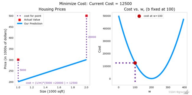
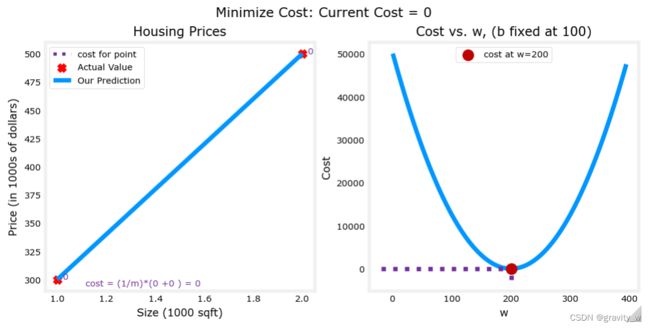
In the previous lab, you determined that $b=100$ provided an optimal solution so let’s set $b$ to 100 and focus on $w$.

plt_intuition(x_train,y_train)

$w$ = 100时

$w$ = 200时

The plot contains a few points that are worth mentioning.

• cost is minimized when $w=200$, which matches results from the previous lab
• Because the difference between the target and prediction is squared in the cost equation, the cost increases rapidly when $w$ is either too large or too small.
• Using the w and b selected by minimizing cost results in a line which is a perfect fit to the data.

Cost Function Visualization-3D

You can see how cost varies with respect to both w and b by plotting in 3D or using a contour plot.
本课程中的一些绘图示例可能会非常复杂，不需要掌握，代码在lab_utils_uni.py中

Larger Data Set

给出一个数据集，其中的数据点不在一条直线上

x_train = np.array([1.0, 1.7, 2.0, 2.5, 3.0, 3.2])
y_train = np.array([250, 300, 480,  430,   630, 730,])

等高线图是可视化3D Cost Function的一种便捷方式
在jupyter notebook中，可以单击等高线图中的一个点来选择 $w$ 和 $b$ 以实现最低成本，更新图形可能需要几秒钟的时间

plt.close('all') 
fig, ax, dyn_items = plt_stationary(x_train, y_train)
updater = plt_update_onclick(fig, ax, x_train, y_train, dyn_items)

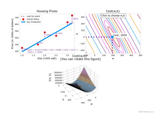
注意图上的虚线，代表了每个实例所贡献的cost，在这种情况下， $w$ = 209和 $b$ = 2.4提供low cost
因为数据点不在一条线上，所以最小cost不是0

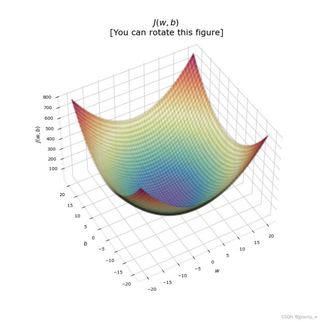
Convex Cost Surface

因为cost function对loss进行平方，所以保证了’error surface’像碗一样凸起，它总是有一个可以在所有维度上使用梯度来达到的最小值
在前面的图中，由于 $w$ 和 $b$ 的尺度不同，所以不易辨认，下面的图中 $w$ 和 $b$ 是对称的，更易辨认

soup_bowl()

Congratulations!

You have learned the following:

• The cost equation provides a measure of how well your predictions match your training data.
• Minimizing the cost can provide optimal values of $w$, $b$.