深度学习(6)--Keras项目详解
目录
一.项目介绍
二.项目流程详解
2.1.导入所需要的工具包
2.2.输入参数
2.3.获取图像路径并遍历读取数据
2.4.数据集的切分和标签转换
2.5.网络模型构建
2.6.绘制结果曲线并将结果保存到本地
三.完整代码
四.首次运行结果
五.学习率对结果的影响
六.Dropout操作对结果的影响
七.权重初始化对结果的影响
7.1.RandomNormal
7.2.TruncatedNormal(推荐)
八.正则化对结果的影响
九.加载模型进行测试
一.项目介绍
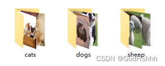
用Keras工具包搭建训练自己的一个传统神经网络,用来识别猫/狗/羊三种图片。
数据集:

二.项目流程详解
2.1.导入所需要的工具包
# 导入所需要的工具包
# 将建模的结果画出来
import matplotlib
# 做标签,数据切分,展示结果的对比
from sklearn.preprocessing import LabelBinarizer
from sklearn.model_selection import train_test_split
from sklearn.metrics import classification_report
# keras工具包的操作
from keras.models import Sequential
from keras.layers import Dropout
# from keras.layers.core import Dense
from tensorflow.python.keras.layers.core import Dense
from keras.optimizers import SGD
from keras import initializers
from keras import regularizers
# 图像路径处理操作
from my_utlis import utlis_paths
# 一些基本库
import matplotlib.pyplot as plt
import numpy as np
import argparse
import random
import pickle
import cv2
import os

os.environ["CUDA_VISIBLE_DEVICES"] = "0"
(1).如果只安装了keras工具包没安装cv2库,可以参考以下链接在Anaconda的虚拟环境中安装cv2库。
https://blog.csdn.net/u011204487/article/details/86497431 https://blog.csdn.net/u011204487/article/details/86497431
(2).如果 from keras.layers.core import Dense 显示此结果
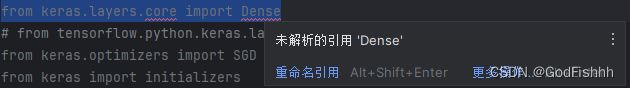
可以将导入代码改为如下方式
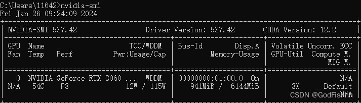
from tensorflow.python.keras.layers.core import Dense(3).在代码开头加入os.environ["CUDA_VISIBLE_DEVICES"] = "0"这行代码可以用gpu训练网络,“0”为可以使用的gpu编号,可以在cmd中输入nvidia -smi查询可用的gpu编号:
2.2.输入参数
# --dataset --model --label-bin --plot
# 输入参数
ap = argparse.ArgumentParser()
ap.add_argument("-d", "--dataset", required=True,
                help="path to input dataset of images")
ap.add_argument("-m", "--model", required=True,
                help="path to output trained model")
ap.add_argument("-L", "--Label-bin", required=True,
                help="path to output label binarizer")
ap.add_argument("-p", "--plot", required=True,
                help="path to output accuracy/loss plot")
args = vars(ap.parse_args())
设置参数
右键项目点击修改运行配置

设置参数的值

设置好参数后在对应处创建文件夹
2.3.获取图像路径并遍历读取数据
# 获取图像数据路径,方便后续读取
imagePaths = sorted(list(utlis_paths.list_images('./dataset')))
random.seed(42)
random.shuffle(imagePaths)

# 遍历读取数据
for imagePath in imagePaths:
    # 读取图像数据,后续步骤中使用了神经网络,需要将图像数据设置成一维
    image = cv2.imread(imagePath)  # cv2.imread方法读取数据
    image = cv2.resize(image, (32, 32)).flatten()  # 将读取的图片数据设置成相同的大小
    data.append(image)

    # 读取标签
    label = imagePath.split(os.path.sep)[-2]
    labels.append(label)

# scale图像数据
data = np.array(data, dtype="float") / 255.0
labels = np.array(labels)
调用utlis_paths.list_images,获取路径的文件
通过from my_utlis import utlis_paths引入utlis_paths,所以需要在my_utlis文件夹中生成一个utlis_paths文件并在其中完成相应的函数定义:
![]()
import os


image_types = (".jpg", ".jpeg", ".png", ".bmp", ".tif", ".tiff")


def list_images(basePath, contains=None):
    # 返回有效的图片路径数据集
    return list_files(basePath, validExts=image_types, contains=contains)


def list_files(basePath, validExts=None, contains=None):
    # 遍历图片数据目录,生成每张图片的路径
    for (rootDir, dirNames, filenames) in os.walk(basePath):
        # 循环遍历当前目录中的文件名
        for filename in filenames:
            # if the contains string is not none and the filename does not contain
            # the supplied string, then ignore the file
            if contains is not None and filename.find(contains) == -1:
                continue

            # 通过确定.的位置,从而确定当前文件的文件扩展名
            ext = filename[filename.rfind("."):].lower()

            # 检查文件是否为图像,是否应进行处理
            if validExts is None or ext.endswith(validExts):
                # 构造图像路径
                imagePath = os.path.join(rootDir, filename)
                yield imagePath
指定一个随机种子,确保每次的切割相同,同时将数据洗牌,打乱数据
random.seed(42)  # 指定随机种子
random.shuffle(imagePaths)  # 把数据重新洗牌,即将数据打乱
读取数据,并将所有的数据设置为统一规格
image = cv2.imread(imagePath)  # cv2.imread方法读取数据
image = cv2.resize(image, (32, 32)).flatten()  # 将读取的图片数据设置成相同的大小
data.append(image)  # append()函数向列表末尾添加一个元素
flatten()函数将图片参数拉长。
eg.32x32x3大小的图片,拉长为3072个像素点,即变为1x3072的矩阵
给读取出来的数据设置标签(读取数据和设置标签一般放在一起)
label = imagePath.split(os.path.sep)[-2]
labels.append(label)
scale归一化获得的图片数据,使得特征值在0~1之间浮动
# scale图像数据
data = np.array(data, dtype="float") / 255.0
2.4.数据集的切分和标签转换
# 数据集切分
(trainX, testX, trainY, testY) = train_test_split(data,
                         labels, test_size=0.25, random_state=42)

# 转换标签,one-hot格式
lb = LabelBinarizer()
trainY = lb.fit_transform(trainY)
testY = lb.transform(testY)
划分训练集和测试集:
(trainX, testX, trainY, testY) = train_test_split(data,
                         labels, test_size=0.25, random_state=42)
函数原型:
X_train, X_test, y_train, y_test = train_test_split(train_data, train_target, test_size, random_state, shuffle)
变量:
X_train:划分的训练集数据
X_test:划分的测试集数据
y_train:划分的训练集标签
y_test:划分的测试集标签
参数:
train_data:还未划分的数据集
train_target:还未划分的标签
test_size:分割比例,默认为0.25,即测试集占完整数据集的比例
random_state:随机数种子,应用于分割前对数据的洗牌。可以是int,RandomState实例或None,默认值=None。设成定值意味着,对于同一个数据集,只有第一次运行是随机的,随后多次分割只要rondom_state相同,则划分结果也相同。
shuffle:是否在分割前对完整数据进行洗牌(打乱),默认为True,打乱
转换标签:
lb = LabelBinarizer()
trainY = lb.fit_transform(trainY)
testY = lb.transform(testY)
最后得到的结果是对应三个动物种类狗、猫、羊的概率值,所以就应当有三个标签,需要对当前的标签进行转换,转换为满足要求的one-hot标签格式。
2.5.网络模型构建
# 网络模型结构 3072-512-256-3
model = Sequential()
# kernel_regularizer=regularizers.12(0.01)
# keras.initializers.TruncatedNormal(mean=0.0, stddex=0.05, seed=None)
# initializers.random_normal
# #model.add(Dropout(0.8))
model.add(keras.Input(shape=(3072,)))
model.add(Dense(512, activation="relu"))
model.add(Dense(256, activation="relu"))
model.add(Dense(len(lb.classes_), activation="softmax",))

# 初始化参数
INIT_LR = 0.01
EPOCHS = 200

# 给定损失函数和评估方法
print("[INFO] 准备训练网络...")
opt = SGD(lr=INIT_LR)
model.compile(loss="categorical_crossentropy", optimizer=opt,
              metrics=["accuracy"])

# 训练网络模型
H = model.fit(trainX, trainY, validation_data=(testX,testY),
              epochs=EPOCHS, batch_size=32)

# 测试网络模型
print("[INFO] 正在评估模型")
predictions = model.predict(testX, batch_size=32)
print(classification_report(testY.argmax(axis=1),
      predictions.argmax(axis=1), target_names=lb.classes_))
该网络模型的共有三层,初始特征值有3072个,由3072-512-256-3,最后得到对应三个图像类别的概率值。
设置模型的类型为Sequential :
model = Sequential()对于Sequential模型的相关信息,可以查询下述keras的官方网站:
https://keras.io/guides/sequential_model/https://keras.io/guides/sequential_model/

向神经网络中添加三层:
第一层:
model.add(keras.Input(shape=(3072,)))
model.add(Dense(512, activation="relu"))
首先第一层一般要通过Input(n,)函数告诉网络起始层有多少个神经元,然后512表示的是转换为下一层的神经元为512个,激活函数设置的是relu。
第二层:
model.add(Dense(256, activation="relu"))经过这一层得到的下一层的神经元应当有256个,同时激活函数设置的为relu。
第三层:
model.add(Dense(len(lb.classes_), activation="softmax",))经过这一层得到下一层的神经元个数为len(lb.classes_)的返回值,此处为3,同时激活函数为softmax,最后得到对应的不同类别的概率值。
初始化参数:
INIT_LR = 0.01
EPOCHS = 200
INIT_LR为学习率,EPOCHS为遍历整个数据集的次数
设置损失函数和评估方法:
opt = SGD(lr=INIT_LR)
model.compile(loss="categorical_crossentropy", optimizer=opt,
              metrics=["accuracy"])
SGD为随机梯度下降,将opt优化器设置为随机梯度下降,同时将学习率告诉SGD。
选择的损失函数为categorical_crossentropy,即为交叉熵损失函数 。
最后再获取accuracy准确率
训练网络模型:
H = model.fit(trainX, trainY, validation_data=(testX,testY),
              epochs=EPOCHS, batch_size=32)
测试网络模型:
print("[INFO] 正在评估模型")
predictions = model.predict(testX, batch_size=32)
print(classification_report(testY.argmax(axis=1),
      predictions.argmax(axis=1), target_names=lb.classes_)))
2.6.绘制结果曲线并将结果保存到本地
# 调试完成后,绘制结果曲线
N = np.arange(0, EPOCHS)
plt.style.use("ggplot")
plt.figure()
plt.plot(N, H.history["loss"], label="train_loss")
plt.plot(N, H.history["val_loss"], label="val_loss")
plt.plot(N, H.history["acc"], label="train_acc")
plt.plot(N, H.history["val_acc"], label="val_acc")
plt.title("Training Loss and Accuracy (Simple NN)")
plt.xlabel("Epoch #")
plt.ylabel("Loss/Accuracy")
plt.legend()
plt.savefig('./output/simple_nn_plot.png')   # 参数为保存的路径

# 保存模型到本地
print("[INFO] 正在保存模型")
model.save(args["model"])
f = open('./output/simple_nn_lb.pickle', "wb")  # 保存标签数据
f.write(pickle.dumps(lb))
f.close()
对于acc参数,不同版本的keras对应的写法不同,如果引入acc和val_acc报错,可以尝试改为accuracy和val_accuracy,反之亦然。
三.完整代码
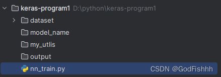
项目结构:
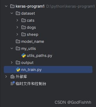
nn_train.py:
# 导入所需要的工具包
# 将建模的结果画出来
import keras
import matplotlib
# 做标签,数据切分,展示结果的对比
from sklearn.preprocessing import LabelBinarizer
from sklearn.model_selection import train_test_split
from sklearn.metrics import classification_report
# keras工具包的操作
from keras.models import Sequential
from keras.layers import Dropout
# from keras.layers.core import Dense
from tensorflow.python.keras.layers.core import Dense
from keras.optimizers import SGD
from keras import initializers
from keras import regularizers
# 图像路径处理操作
from my_utlis import utlis_paths
# 一些基本库
import matplotlib.pyplot as plt
import numpy as np
import argparse
import random
import pickle
import cv2
import os

# --dataset --model --label-bin --plot
# 输入参数
ap = argparse.ArgumentParser()
ap.add_argument("-d", "--dataset", required=True,
                help="path to input dataset of images")
ap.add_argument("-m", "--model", required=True,
                help="path to output trained model")
ap.add_argument("-L", "--Label-bin", required=True,
                help="path to output label binarizer")
ap.add_argument("-p", "--plot", required=True,
                help="path to output accuracy/loss plot")
args = vars(ap.parse_args())


print("[INFO] 开始读取数据")
data = []
labels = []

# 获取图像数据路径,方便后续读取
imagePaths = sorted(list(utlis_paths.list_images('./dataset')))
random.seed(42)  # 指定随机种子
random.shuffle(imagePaths)  # 把数据重新洗牌,即将数据打乱

# 遍历读取数据
for imagePath in imagePaths:
    # 读取图像数据,后续步骤中使用了神经网络,需要将图像数据设置成一维
    image = cv2.imread(imagePath)  # cv2.imread方法读取数据
    image = cv2.resize(image, (32, 32)).flatten()  # 将读取的图片数据设置成相同的大小
    data.append(image)

    # 读取标签
    label = imagePath.split(os.path.sep)[-2]
    labels.append(label)

# scale图像数据
data = np.array(data, dtype="float") / 255.0
labels = np.array(labels)

# 数据集切分
(trainX, testX, trainY, testY) = train_test_split(data,
                         labels, test_size=0.25, random_state=42)

# 转换标签,one-hot格式
lb = LabelBinarizer()
trainY = lb.fit_transform(trainY)
testY = lb.transform(testY)

# 网络模型结构 3072-512-256-3
model = Sequential()
# kernel_regularizer=regularizers.12(0.01)
# keras.initializers.TruncatedNormal(mean=0.0, stddex=0.05, seed=None)
# initializers.random_normal
# #model.add(Dropout(0.8))
model.add(keras.Input(shape=(3072,)))
model.add(Dense(512, activation="relu"))
model.add(Dense(256, activation="relu"))
model.add(Dense(len(lb.classes_), activation="softmax",))

# 初始化参数
INIT_LR = 0.01
EPOCHS = 200

# 给定损失函数和评估方法
print("[INFO] 准备训练网络...")
opt = SGD(lr=INIT_LR)
model.compile(loss="categorical_crossentropy", optimizer=opt,
              metrics=["accuracy"])

# 训练网络模型
H = model.fit(trainX, trainY, validation_data=(testX,testY),
              epochs=EPOCHS, batch_size=32)

# 测试网络模型
print("[INFO] 正在评估模型")
predictions = model.predict(testX, batch_size=32)
print(classification_report(testY.argmax(axis=1),
      predictions.argmax(axis=1), target_names=lb.classes_))

# 调试完成后,绘制结果曲线
N = np.arange(0, EPOCHS)
plt.style.use("ggplot")
plt.figure()
plt.plot(N, H.history["loss"], label="train_loss")
plt.plot(N, H.history["val_loss"], label="val_loss")
plt.plot(N, H.history["accuracy"], label="train_acc")
plt.plot(N, H.history["val_accuracy"], label="val_acc")
plt.title("Training Loss and Accuracy (Simple NN)")
plt.xlabel("Epoch #")
plt.ylabel("Loss/Accuracy")
plt.legend()
plt.savefig('./output/simple_nn_plot.png')   # 参数为保存的路径

# 保存模型到本地
print("[INFO] 正在保存模型")
model.save(args["model"])
f = open('./output/simple_nn_lb.pickle', "wb")  # 保存标签数据
f.write(pickle.dumps(lb))
f.close()
utlis_paths.py:
import os
image_types = (".jpg", ".jpeg", ".png", ".bmp", ".tif", ".tiff")
def list_images(basePath, contains=None):
# 返回有效的图片路径数据集
return list_files(basePath, validExts=image_types, contains=contains)
def list_files(basePath, validExts=None, contains=None):
# 遍历图片数据目录,生成每张图片的路径
for (rootDir, dirNames, filenames) in os.walk(basePath):
# 循环遍历当前目录中的文件名
for filename in filenames:
# if the contains string is not none and the filename does not contain
# the supplied string, then ignore the file
if contains is not None and filename.find(contains) == -1:
continue
# 通过确定.的位置,从而确定当前文件的文件扩展名
ext = filename[filename.rfind("."):].lower()
# 检查文件是否为图像,是否应进行处理
if validExts is None or ext.endswith(validExts):
# 构造图像路径
imagePath = os.path.join(rootDir, filename)
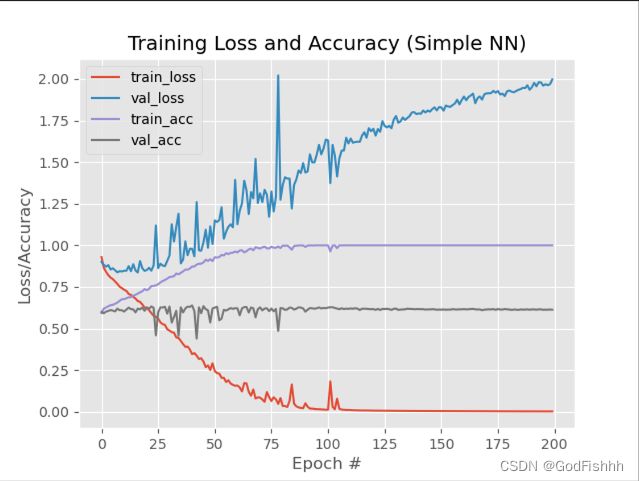
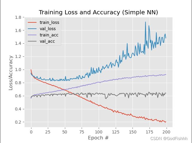
yield imagePath四.首次运行结果

相关参数介绍参考文章:
https://blog.csdn.net/weixin_48964486/article/details/122881350

在训练集上的accuracy为1.0,与测试集上的accuracy差距过大,可能出现过拟合现象。
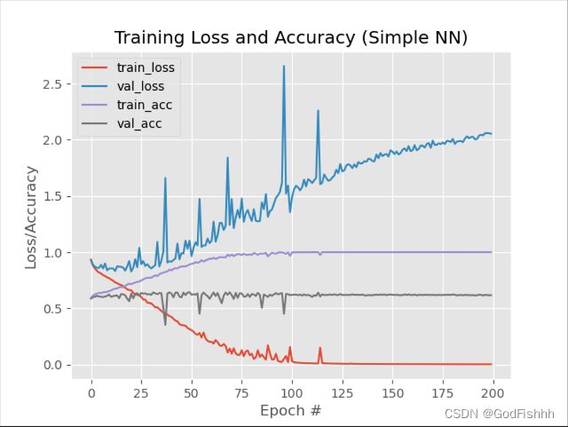
五.学习率对结果的影响
初始学习率为0.01(学习率过大可能产生过拟合现象)
将学习率改为0.001:
# 初始化参数
INIT_LR = 0.001
EPOCHS = 200
训练结果: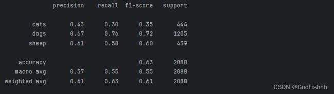

仍有过拟合现象,但是相较于学习率lr=0.01的情况略有改善。
六.Dropout操作对结果的影响
The Dropout layer randomly sets input units to 0 with a frequency of rate at each step during training time, which helps prevent overfitting
Dropout layer (keras.io)https://keras.io/api/layers/regularization_layers/dropout/
添加Drop-out操作:
一般添加在全连接层中
from keras.layers import Dropout

model.add(keras.Input(shape=(3072,)))
model.add(Dense(512, activation="relu"))
model.add(Dropout(0.5))
model.add(Dense(256, activation="relu"))
model.add(Dropout(0.5))
model.add(Dense(len(lb.classes_), activation="softmax",))
Dropout=0.5,LR=0.001的训练结果:


从结果可以看出,添加Dropout层可以有效避免过拟合现象的出现。
七.权重初始化对结果的影响
查询不同的初始化方法:
Layer weight initializers (keras.io)https://keras.io/api/layers/initializers/查看全连接层的参数设置发现,如果不初始化kernel_initializer,起默认的参数为'glorot_uniform',即正态分布初始化,常常不能满足训练的要求。

7.1.RandomNormal
将kernel_initializer设置为‘RandomNormal’,即高斯正太分布:
from keras import initializers

model.add(keras.Input(shape=(3072,)))
model.add(Dense(512, activation="relu", kernel_initializer=keras.initializers.RandomNormal(mean=0.0, stddev=0.05, seed=None)))
# model.add(Dropout(0.5))
model.add(Dense(256, activation="relu", kernel_initializer=keras.initializers.RandomNormal(mean=0.0, stddev=0.05, seed=None)))
# model.add(Dropout(0.5))
model.add(Dense(len(lb.classes_), activation="softmax", kernel_initializer=keras.initializers.RandomNormal(mean=0.0, stddev=0.05, seed=None)))
其中mean为均值,stddev为标准差。
正太高斯分布初始化,不使用Dropout层,LR=0.001的训练结果:

7.2.TruncatedNormal(推荐)
将kernel_initializer设置为‘TruncatedNormal’,即截断正太分布:
model.add(keras.Input(shape=(3072,)))
model.add(Dense(512, activation="relu", kernel_initializer=keras.initializers.TruncatedNormal(mean=0.0, stddev=0.05, seed=None)))
# model.add(Dropout(0.5))
model.add(Dense(256, activation="relu", kernel_initializer=keras.initializers.TruncatedNormal(mean=0.0, stddev=0.05, seed=None)))
# model.add(Dropout(0.5))
model.add(Dense(len(lb.classes_), activation="softmax", kernel_initializer=keras.initializers.TruncatedNormal(mean=0.0, stddev=0.05, seed=None)))
其中mean为均值,stddev为标准差。
截断正太分布初始化,不使用Dropout层,LR=0.001的训练结果:

在此基础上再加上Dropout层的结果:
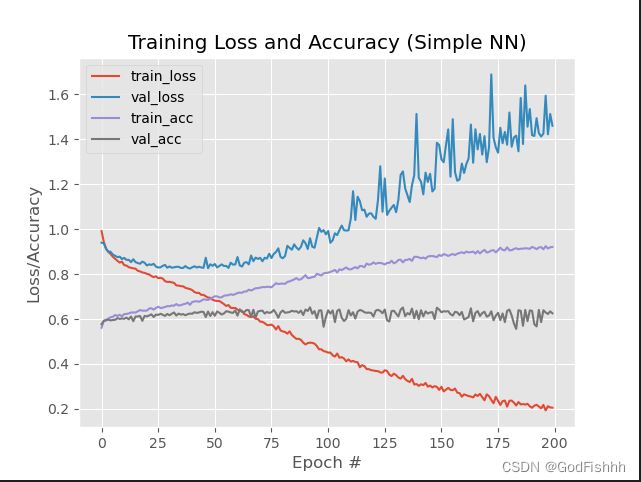
八.正则化对结果的影响
Regularizers allow you to apply penalties on layer parameters or layer activity during optimization. These penalties are summed into the loss function that the network optimizes.
Layer weight regularizers (keras.io)https://keras.io/api/layers/regularizers/
在全连接层添加正则化:
from keras import regularizers

model.add(keras.Input(shape=(3072,)))
model.add(Dense(512, activation="relu", kernel_initializer=keras.initializers.TruncatedNormal(mean=0.0, stddev=0.05, seed=None), kernel_regularizer=regularizers.L2(0.01)))
model.add(Dropout(0.5))
model.add(Dense(256, activation="relu", kernel_initializer=keras.initializers.TruncatedNormal(mean=0.0, stddev=0.05, seed=None), kernel_regularizer=regularizers.L2(0.01)))
model.add(Dropout(0.5))
model.add(Dense(len(lb.classes_), activation="softmax", kernel_initializer=keras.initializers.TruncatedNormal(mean=0.0, stddev=0.05, seed=None), kernel_regularizer=regularizers.L2(0.01)))
有两种正则化方法,L1为取绝对值,L2是求权重的欧几里得范数(常用L2),括号里的参数为惩罚力度 (越大的惩罚力度,过拟合的风险越低)。
惩罚力度为0.01正则化,截断正态分布初始化,加入Dropout=0.5,LR=0.001的训练结果:


惩罚力度为0.1正则化,截断正态分布初始化,加入Dropout=0.5,LR=0.001的训练结果:

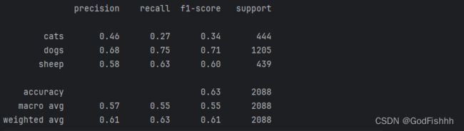
九.加载模型进行测试
保存模型到本地:
保存的模型:惩罚力度为0.1正则化,截断正态分布初始化,加入Dropout=0.5,LR=0.001,EPOCHS=1000.
# 保存模型到本地
print("[INFO] 正在保存模型")
model.save(args["model"])
f = open('./output/simple_nn_lb.pickle', "wb")  # 保存标签数据
f.write(pickle.dumps(lb))
f.close()

编写一个predict.py程序来加载模型进行测试:
# 导入所需工具包
from keras.models import load_model
import argparse
import pickle
import cv2


# 加载测试数据并进行相同预处理操作
image = cv2.imread('./cs_image/dog.jpeg')  # 读取一张图片进行测试 dog/cat/sheet
output = image.copy()  # 复制图片的一份副本给output
image = cv2.resize(image, (32, 32))

# scale图像数据
image = image.astype("float") / 255.0

# 对图像进行拉平操作
image = image.flatten()
image = image.reshape((1, image.shape[0]))

# 读取模型和标签
print("------读取模型和标签------")
model = load_model('./output/simple_nn.model')  # 设置模型
lb = pickle.loads(open('./output/simple_nn_lb.pickle', "rb").read())  # 设置标签

# 预测
preds = model.predict(image)

# 得到预测结果以及其对应的标签
i = preds.argmax(axis=1)[0]
label = lb.classes_[i]

# 在图像中把结果画出来
text = "{}: {:.2f}%".format(label, preds[0][i] * 100)
cv2.putText(output, text, (10, 30), cv2.FONT_HERSHEY_SIMPLEX, 0.7,(0, 0, 255), 2)

# 绘图
cv2.imshow("Image", output)
cv2.waitKey(0)
若出现下述报错
error: (-2:Unspecified error) The function is not implemented. Rebuild the library with Windows, GTK+ 2.x or Cocoa support.在对应的虚拟环境中安装OpenCV的拓展开发包即可解决
pip install opencv-contrib-python -i https://pypi.tuna.tsinghua.edu.cn/simple/
测试的结果:


发现对于猫的预测结果不准确,对于图片的预测,一般会用到卷积神经网络而不是本项目中构建的传统神经网络。