Auto-Encoding Variational Bayes整理

Auto-Encoding Variational Bayes

How can we perform efficient inference and learning in directed probabilistic models, in the presence of continuous latent variables with intractable posterior distributions, and large datasets?

introduce a stochastic variational inference and learning algorithm that scales to large datasets and, under some mild differentiability conditions, even works in the intractable case.

contributions is two-fold.

• a reparameterization of the variational lower bound yields a lower bound estimator that can be straightforwardly optimized using standard stochastic gradient methods.
  对变分下界的重新参数化得到一个下界估计量，该下界估计量可以用标准随机梯度法直接优化。
• for i.i.d. datasets with continuous latent variables per datapoint, posterior inference can be made especially efficient by fitting an approximate inference model (also called a recognition model) to the intractable posterior using the proposed lower bound estimator.
  对于每个数据点具有连续潜在变量的i.i.d.数据集，通过使用所提出的下界估计器将一个近似推理模型（也称为识别模型）拟合到难以处理的后验，可以使后验推理变得尤其有效

在自编码网络中，从 $x\to z\to x^{\prime }$ ，这样一个过程，实现无监督表征学习， $z$ 是自动学习的，没有任何的先验约束，但是在有时候，希望符合某个分布，也就是实现无监督表征空间 $z$ 的约束。
变分自编码器的算法实现挺简单，只是在损失函数中 加入了一个正则约束，用于约束高维空间的隐变量 $z$ 满足高斯分布。其推导过程可不简单。

---

introduction

We show how a reparameterization of the variational lower bound yields a simple differentiable unbiased estimator of the lower bound; this SGVB (Stochastic Gradient Variational Bayes) estimator can be used for efficient approximate posterior inference in almost any model with continuous latent variables and/or parameters, and is straightforward to optimize using standard stochastic gradient ascent techniques.
我们展示了变分下界的重参数化如何产生下界的简单可微的无偏估计;这种SGVB（随机梯度变异贝叶斯）估计器可以用于几乎任何具有连续隐变量和/或参数的模型中的有效近似后验推理，并且可以直接使用标准随机梯度上升技术进行优化

For the case of an i.i.d. dataset and continuous latent variables per datapoint, we propose the AutoEncoding VB (AEVB) algorithm . In the AEVB algorithm we make inference and learning especially efficient by using the SGVB estimator to optimize a recognition model that allows us to perform very efficient approximate posterior inference using simple ancestral sampling, which in turn allows us to efficiently learn the model parameters, without the need of expensive iterative inference schemes (such as MCMC) per datapoint.
对于i.i.d.数据集和每个数据点的连续隐变量的情况，我们提出了自动编码变分贝叶斯VB（AEVB）算法。在AEVB算法中，我们通过使用SGVB估计器来优化识别模型，使得我们能够使用简单的原始抽样来执行非常有效的近似后推理，从而使推理和学习特别有效，这反过来又允许我们有效地学习模型参数，而没有每个数据点需要昂贵的迭代推理方案（如MCMC）。

---

method

a lower bound estimator (a stochastic objective function) for a variety of directed graphical models with continuous latent variables.
具有连续隐变量的各种定向图形模型导出下限估计器（随机目标函数）

we have an i.i.d. dataset with latent variables per datapoint, and where we like to perform maximum likelihood (ML) or maximum a posteriori (MAP) inference on the (global) parameters, and variational inference on the latent variables.
我们有一个i.i.d. 数据集与每个数据点的隐变量，我们要对（全局）参数执行最大似然（ML）或最大后验（MAP）推理，以及对隐变量的变分推理。

问题描述

• 生成模型中，样本数据 $X={x^{(i)}}_{i=1}^N$ 包含 $N$ 个连续或者离散的变量 $x$ 的 $i.i.d$ 样本
• 假设样本数据是根据某个随机过程关于一个不可观测到的连续随机变量 $z$ 独立采样生成的
• 数据采样生成过程分为两步：
  1. 由先验分布 $p_{{\theta }^{\ast }}(z)$ 生成 $z^{(i)}$
  2. 由条件分布 $p_{{\theta }^{\ast }}(x\mid z)$ 生成 $x^{(i)}$
     即：$$z^{(i)}\sim p_{{\theta }^{\ast }}(z)$$$$x^{(i)}\sim p_{{\theta }^{\ast }}(x\mid z)$$

$p_{{\theta }^{\ast }}(z)$ 和 $p_{{\theta }^{\ast }}(x\mid z)$ 是一个参数化的概率密度函数(PDF)，取自于参数分布族$p_{\theta }(z)$ 和 $p_{\theta }(x\mid z)$，它们的 $PDFs$ 在 $\theta$ 和 $z$ 上几乎处处可微。但是，真正的参数 ${\theta }^{\ast }$ 以及潜在变量 $z^{(i)}$ 的值我们是未知的。

---

we are here interested in a general algorithm that even works efficiently in the case of:

1. Intractability
2. A large dataset
   
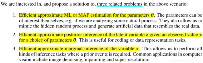
   For the purpose of solving the above problems, let us introduce a recognition model $q_{\varphi }(z\mid x)$ : an approximation to the intractable true posterior $p_{\theta }(z\mid x)$.

Note that in contrast with the approximate posterior in mean-field variational inference, it is not necessarily factorial and its parameters $\varphi$ are not computed from some closed-form expectation. Instead, we’ll introduce a method for learning the recognition model parameters $\varphi$ jointly with the generative model parameters $\theta$.
介绍一种学习识别模型参数 $\varphi$ 和生成模型参数 $\theta$ 的方法。

从编码理论的角度来看，未观测到的变量 $z$ 被解释为一个潜在变量表示或编码。在本文中，我们也将把识别模型 $q_{\varphi }(z\mid x)$ 称为 概率编码器(a probabilistic encoder)，因为给定一个数据点 $x$ ，它会在编码 $z$ 的可能值上产生一个分布（例如高斯分布），从中可以生成数据点 $x$ 。类似地，我们将把 $p_{\theta }(x\mid z)$ 称为 概率解码器(a probabilistic decoder)，因为给定一个编码 $z$ ，它会在 $x$ 的可能对应值上产生一个分布。

推导变分下界

边缘似然由单个数据点的边缘似然之和组成：$$log{p}_{\theta }(x^1,...,x^N)=\sum _{i=1}^{N}log{p}_{\theta }(x^i)$$

自编码, 通过引入Encoder和Decoder来估计联合分布 $p(x,z)$ , 其中表示隐变量(我们也可以让 $z$ 为样本标签, 使得Encoder成为一个判别器).
在Decoder中我们 建立 $p_{\theta }(x,z)$ 联合分布以估计 $p(x,z)$ , 在Encoder中建立一个后验分布 $q_{\varphi }(z\mid x)$ 去估计 $p_{\theta }(z\mid x)$ , 然后极大似然:

上式俩边关于z在分布 $q_{\varphi }(z)$ 下求期望可得:

原文中有：

既然KL散度非负, 我们极大似然$\log p_{\theta }(x)$可以退而求其次, 最大化${\mathbb{E}}_{q_{\varphi }(z|x)}(\log \frac{p_{\theta }(x,z)}{q_{\varphi }(z|x)})$(ELBO, 记为$\mathcal{L}$).

也就是变分编码器下界：

又($p_{\theta }(z)$为认为给定的先验分布)
最大化似然函数，也可以直接最大化 $L(\theta ,\varphi ;x)$ 来提高变分下界。

---

求解该公式的最大值，就需要用梯度上升（或者梯度下降）更新，那么就需要求导。
$\mathcal{L}$ 的第一项是KL惩罚项，用于约束自编码器的编码向量 $z$ 尽量逼近于先验分布 $p(z)$， 衡量近似后验概率分布函数与先验分布的相似性，通过此项防止过拟合。第二项是对数似然估计，可以看成是自编码器误差损失重构项，$q(z\mid x)$ 相当于给定样本 $x$ 输出编码 $z$，$p(x\mid z)$ 相当于解码输出重构样本 $x$。
$q(z\mid x)$相当于编码过程， $p(x\mid z)$ 相当于解码过程。

---

Encoder (损失part1)

Encoder 将 $x\to z$, 就相当于在 $q_{\varphi }(z|x)$ 中进行采样, 但是如果是直接采样的话, 就没法利用梯度回传进行训练了, 这里需要一个重参化技巧。

• 假设 $q_{\varphi }(z|x)$ 为高斯密度函数, 即 $\mathcal{N}(\mu ,{\sigma }^{2}I)$

构建一个神经网络 $f$ , 其输入为样本 $x$ , 输出为 $(\mu ,\log \sigma )$ (输出 $\log \sigma$是为了保证 $\sigma$ 为正), 则
$$z=\mu +ϵ\odot \sigma ,ϵ\sim \mathcal{N}(0,I)$$其中 $\odot$ 表示按元素相乘。
注: 我们可以该输出为 $(\mu ,L)$ ( $L$ 为三角矩阵, 且对角线元素非负), 而假设 $q_{\varphi }(z|x)$ 的分量不独立, 其协方差函数为 $L^{T}L$ , 则$(z=\mu +Lϵ).$

---

变分下界第一项

当 $p_{\theta }(z)=\mathcal{N}(0,I)$ , 我们可以显示表达出:


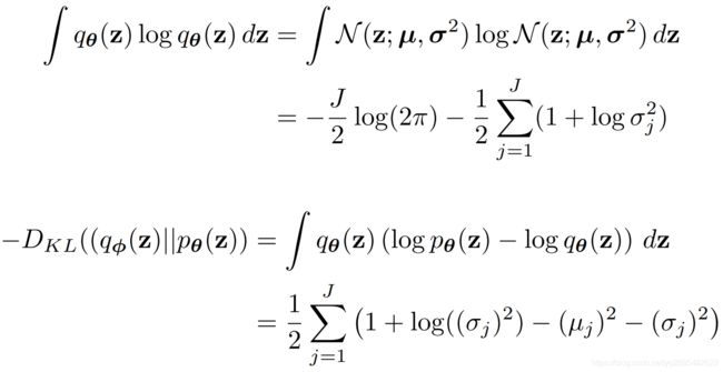
那么根据复合函数求导法则:如果对这一项进行求导(关于编码网络层参数 $\varphi$ 的偏导数)，其实也就是对 $(\mu ,\sigma )$进行求导，进而对编码层的网络参数 $\varphi$ 进行求导；用梯度下降法BP更新，就可以了。因此对于这一项惩罚项来说，用梯度下降法问题不大，该怎么求导还是怎么求导，真正问题大条的是变分下界的第二项。

Decoder (损失part2)

Decoder部分, 我们可以通过给定一个 $z$ 然后获得一个 $\hat{x}$

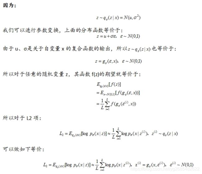
变分下界第二项

这一项是一个对数似然期望，如果也是根据变分下界第一项的推导方法进行推导、积分，会很复杂，在机器学习领域，对于求解复杂积分期望问题，可以采用MC算法。也就是我们可以通过从分布函数q中，采样足够多的样本求取平均值，来近似这一项。然而这个过程是一个不可微的过程，导致无法求取参数的导数，主要原因在于采样过程取决于模型参数。采用这种方法来估计梯度值，会出现很大的偏差，不可行。
然后使用重参数化技巧，进行参数变换：

附

Auto-Encoding Variational Bayes
深度学习（五十一）变分贝叶斯自编码器(上)
深度学习（五十二）变分贝叶斯自编码器(下)