用机器学习方法来预测设备故障
最近做了一个项目,根据设备的状态,来判断设备是否有故障,这里总结一下所用到的数据探索,特征工程以及机器学习模型等方法。考虑到项目数据的敏感性,这里我以网上找到的一个公开数据集UCI Machine Learning Repository作为示例,其中用到的方法和我项目中所用到的方法是一致的。
数据探索
首先我们先对数据集探索一下,看一下包括了哪些特征以及特征的分布情况。这里都是采用Pandas和matplotlib来对数据进行探索
先看一下训练集的数据情况
train_df = pd.read_csv('train.csv')
train_df.info()
输出如下:
Data columns (total 14 columns):
 #   Column                   Non-Null Count   Dtype
---  ------                   --------------   -----
 0   id                       136429 non-null  int64
 1   Product ID               136429 non-null  object
 2   Type                     136429 non-null  object
 3   Air temperature [K]      136429 non-null  float64
 4   Process temperature [K]  136429 non-null  float64
 5   Rotational speed [rpm]   136429 non-null  int64
 6   Torque [Nm]              136429 non-null  float64
 7   Tool wear [min]          136429 non-null  int64
 8   Machine failure          136429 non-null  int64
 9   TWF                      136429 non-null  int64
 10  HDF                      136429 non-null  int64
 11  PWF                      136429 non-null  int64
 12  OSF                      136429 non-null  int64
 13  RNF                      136429 non-null  int64
可见训练集共有136429条数据,数据字段没有缺失值,其中Machine failure表示设备是否有故障。
我们可以查看一下头5条数据
train_df.head(5)输出如下:
从特征值可以看到,id和Product ID可以排除,Air Temperature, Process temperature, Rotational speed, Torque, Tool wear这几个特征是连续值,其他特征是分类值。
连续值特征分析
先对连续值的特征进行一些探索,看看数据的分布情况和Machine Failure之间的联系。
首先我们需要把训练集按照是否有Failure来进行分组,如以下代码:
grouped = train_df.groupby(train_df['Machine failure'])
group0 = grouped.get_group(0)
group1 = grouped.get_group(1)
然后我们对Air Temperature这个特征进行分析并以图形展示,如以下代码:
fig = plt.figure(figsize=(16, 12))
plot_rows = 3
plot_cols = 2
ax1 = plt.subplot2grid((plot_rows,plot_cols), (0,0), rowspan=1, colspan=1)
plt.hist(
    [group0['Air temperature [K]'], group1['Air temperature [K]']],
    bins=10,
    stacked = False,
    label=['No Failure', 'Failure'], alpha = .6)
plt.legend(loc='best', fontsize='x-small')
ax1.set_title('Failure distribution by air temperature')
ax1.set_yscale('log')
#----
ax2 = plt.subplot2grid((plot_rows,plot_cols), (0,1), rowspan=1, colspan=1)
plt.boxplot(
    [group0['Air temperature [K]'], group1['Air temperature [K]']],
    labels=['No Failure', 'Failure'])
plt.legend(loc='best', fontsize='x-small')
ax2.set_title('Failure box plot by air temperature')
#----
ax3 = plt.subplot2grid((plot_rows,plot_cols), (1,0), rowspan=1, colspan=1)
plt.hist(
    [group1['Air temperature [K]']],
    bins=10,
    stacked = False,
    density= True,
    label=['Failure'], alpha = .6)
ax3.set_title('Density hist plot by air temperature for failures')
#----
ax4 = plt.subplot2grid((plot_rows,plot_cols), (1,1), rowspan=1, colspan=1)
plt.hist(
    [train_df['Air temperature [K]']],
    bins=20,
    stacked = False,
    density= False,
    alpha = .6)
ax4.set_title('Distribution or air temperature')
结果如下:
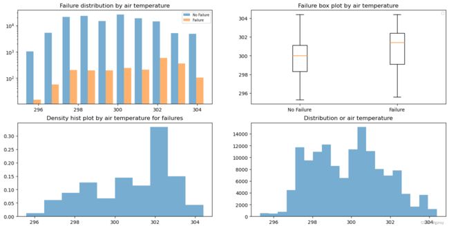
从图中可以看到当温度在302左右时故障较多,对应有故障和无故障的温度分布规律有差异,整体的温度分布大致符合正态分布。
用类似的代码可以看到另外几个连续值特征的分析。
Process Temperature

Rotational speed

Torque

Tool wear
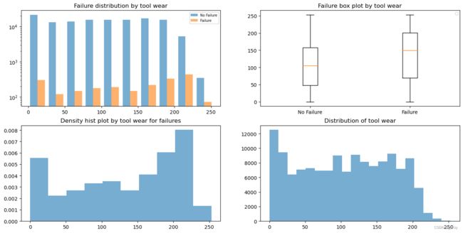
从以上图表中可以对每一个连续值特征的数据分布做分析,这样可以方便我们之后对连续值数据进行处理,例如做归一化的处理,对于数据分布比较符合正态分布,或者异常值较多的,我们可以用 Z score处理,数据分布比较平均的可以用Max/Min来做归一。
离散值特征分析
下面对离散值特征来做数据探索。这里我选择饼图来进行查看,例如以下代码对Type这个特征值做分析
fig = plt.figure(figsize=(16, 10))
plot_rows = 3
plot_cols = 2
ax1 = plt.subplot2grid((plot_rows,plot_cols), (0,0), rowspan=3, colspan=1)
plt.pie(train_df.groupby(train_df['Type']).size(), labels=train_df.groupby(train_df['Type']).indices, autopct='%1.1f%%')
plt.legend(loc='best', fontsize='x-small')
ax1.set_title('Type distribution')
###
ax2 = plt.subplot2grid((plot_rows,plot_cols), (0,1), rowspan=1, colspan=1)
data = train_df.groupby(['Type', 'Machine failure']).size()
plt.pie(data.loc['H'], labels=data.loc['H'].index, autopct='%1.1f%%')
plt.legend(loc='best', fontsize='x-small')
ax2.set_title('Type H distribution')
###
ax3 = plt.subplot2grid((plot_rows,plot_cols), (1,1), rowspan=1, colspan=1)
plt.pie(data.loc['L'], labels=data.loc['L'].index, autopct='%1.1f%%')
plt.legend(loc='best', fontsize='x-small')
ax3.set_title('Type L distribution')
###
ax4 = plt.subplot2grid((plot_rows,plot_cols), (2,1), rowspan=1, colspan=1)
plt.pie(data.loc['M'], labels=data.loc['M'].index, autopct='%1.1f%%')
plt.legend(loc='best', fontsize='x-small')
ax4.set_title('Type M distribution')
结果如下:

可以看到对于每种不同类型,故障率的占比都是差不多的,因此可以初步推测Type这个特征对于判断机器故障用处不大。
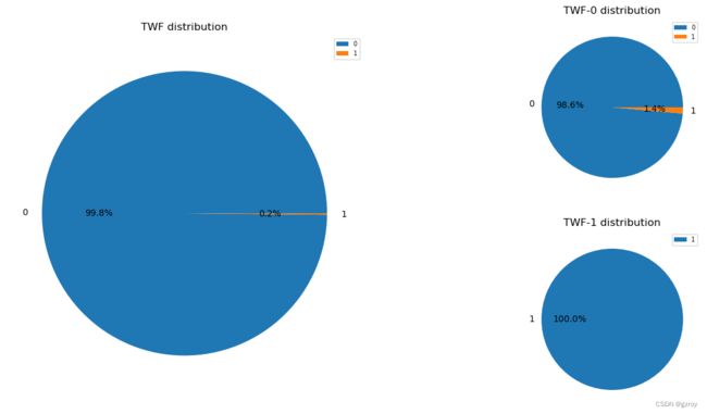
TWF
HDF

PWF

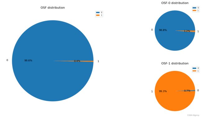
OSF
RNF

以上图表可以很好的了解离散值特征的分布以及其对故障率的影响。
特征相关性
我们还可以对特征之间的相关性进行分析,如果两个特征之间高度相关,那么我们其实可以去掉一个特征,减低模型的复杂性。另外对于高度不相关的特征,我们还可以进行特征组合来创造新的特征。
以下代码可以计算特征之间的皮尔逊相关度:
train_df.drop(columns=['id', 'Machine failure']).corr(method='pearson')输出如下:
	Air temperature [K]	Process temperature [K]	Rotational speed [rpm]	Torque [Nm]	Tool wear [min]	TWF	HDF	PWF	OSF	RNF
Air temperature [K]	1.000000	0.856080	0.016545	-0.006773	0.016994	0.003826	0.100454	0.007967	0.007842	0.004815
Process temperature [K]	0.856080	1.000000	0.011263	-0.006298	0.012777	0.004459	0.041454	0.003871	0.005337	0.004399
Rotational speed [rpm]	0.016545	0.011263	1.000000	-0.779394	0.003983	-0.005765	-0.081996	0.053948	-0.061376	-0.003410
Torque [Nm]	-0.006773	-0.006298	-0.779394	1.000000	-0.003148	0.012983	0.100773	0.050289	0.108765	0.007986
Tool wear [min]	0.016994	0.012777	0.003983	-0.003148	1.000000	0.046470	0.011709	0.007624	0.063604	-0.002071
TWF	0.003826	0.004459	-0.005765	0.012983	0.046470	1.000000	0.010145	0.039927	0.036041	0.002044
HDF	0.100454	0.041454	-0.081996	0.100773	0.011709	0.010145	1.000000	0.046680	0.067149	0.000885
PWF	0.007967	0.003871	0.053948	0.050289	0.007624	0.039927	0.046680	1.000000	0.090016	0.000827
OSF	0.007842	0.005337	-0.061376	0.108765	0.063604	0.036041	0.067149	0.090016	1.000000	-0.000539
RNF	0.004815	0.004399	-0.003410	0.007986	-0.002071	0.002044	0.000885	0.000827	-0.000539	1.000000
我们可以可视化一下:
fig = plt.figure(figsize=(12, 12))
plt.matshow(train_df.drop(columns=['id', 'Machine failure']).corr(method='pearson'), fignum=fig.number)
plt.xticks(range(corr_matrix.columns.shape[0]), corr_matrix.columns, fontsize=8, rotation=45)
plt.yticks(range(corr_matrix.columns.shape[0]), corr_matrix.columns, fontsize=8)
cb = plt.colorbar()
cb.ax.tick_params(labelsize=8)
#plt.title('Correlation Matrix', fontsize=16)
plt.show()
图表如下:
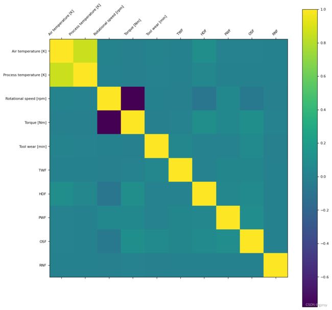
可以看到Air temperature和Process temperature是密切相关的。
基准模型
在进行特征工程之前,我们先看一下基于现有特征,用一个最简单的随机森林模型作为基准模型,看看能达到什么样的性能。
因为特征Type里面包含的是字符,首先我们需要先转换为离散值,如以下代码:
type_to_int = {'H': 0, 'M': 1, 'L': 2}
train_df['TypeInt'] = train_df['Type'].map(type_to_int)
test_df['TypeInt'] = test_df['Type'].map(type_to_int)
把训练集进行划分为训练和测试数据
columns = ['TypeInt', 'Air temperature [K]', 'Process temperature [K]', 'Rotational speed [rpm]', 'Torque [Nm]', 'TWF', 'HDF', 'PWF', 'OSF', 'RNF']
X_train, X_test, y_train, y_test = train_test_split(train_df[columns], train_df['Machine failure'], test_size=0.2, random_state=123)
建立一个简单的随机森林模型来进行训练
rfc = RandomForestClassifier(n_estimators=150, criterion='gini', max_depth=10,
        min_samples_split=2, min_samples_leaf=1, min_weight_fraction_leaf=0.0,
        max_features='auto', max_leaf_nodes=None, bootstrap=True,
        oob_score=False, n_jobs=1, random_state=232, verbose=0, warm_start=False, class_weight=None)
rfc.fit(X_train, y_train)
然后对测试数据进行预测,计算其准确率
result = rfc.predict(X_test)
rightnum = 0

for i in range(0, result.shape[0]):
    if result[i] == y_test.iloc[i]:
        rightnum += 1
print(rightnum/result.shape[0])
可见准确率为99.5932%。这个指标看上去很好,但是考虑到机器故障的只占极小部分,因此用准确率无法反映出模型的性能,我们需要改用精确率和召回率来计算。
精确率的定义为模型判断为有故障的数据中,真正是有故障的数据的占比,即TP/(TP+FP)。召回率的定义为所有有故障的数据中,模型真正能找到的有多少个,即TP/(TP+FN)。F1分数是2*Precision*Recall/(Precision+Recall)。ROC曲线则是判断二元分类模型性能最常用的指标,计算ROC曲线的面积AUC,可以直观的判断模型的性能。以下代码是计算上述的指标:
from sklearn.metrics import roc_auc_score

true_positive = 0
false_negative = 0
false_positive = 0

for i in range(0, result.shape[0]):
    if y_test.iloc[i] == 1:
        if result[i] == 1:
            true_positive += 1
        else:
            false_negative += 1
    else:
        if result[i] == 1:
            false_positive += 1

precision = true_positive/(true_positive + false_positive)
recall = true_positive/(true_positive + false_negative)
f1_score = 2*precision*recall/(precision+recall)
print('Presision: %.4f, Recall: %.4f, F1: %.4f, AUC: %.4f' % (precision, recall, f1_score, roc_auc_score(y_test, result)))
最终的结果为:
Presision: 0.9970, Recall: 0.7528, F1: 0.8579, AUC: 0.9556可以看到,这个模型的精确度不错,但是召回率比较低,所以模型整体的表现一般。
特征工程
根据之前的特征探索,我们可以进行一些特征工程的处理。
连续值的缩放
首先是对连续值特征的处理,虽然随机森林模型不要求对连续值特征缩放到某个区间,但是其他很多模型是对数值区间有要求的,即不同特征的取值区间最好都能统一在同一个范围。这里我采用z score的方式来进行缩放。
train_df = train_df.rename(columns = {
    'Air temperature [K]': 'air_temp',
    'Process temperature [K]': 'process_temp',
    'Rotational speed [rpm]': 'rotational_speed',
    'Torque [Nm]': 'torque',
    'Tool wear [min]': 'tool_wear'}
)
test_df = test_df.rename(columns = {
    'Air temperature [K]': 'air_temp',
    'Process temperature [K]': 'process_temp',
    'Rotational speed [rpm]': 'rotational_speed',
    'Torque [Nm]': 'torque',
    'Tool wear [min]': 'tool_wear'}
)

scaler = StandardScaler()
numeric_columns = ['air_temp', 'process_temp', 'rotational_speed', 'torque', 'tool_wear']
scaler.fit(train_df[numeric_columns])
train_transformed = scaler.transform(train_df[numeric_columns])
test_transformed = scaler.transform(test_df[numeric_columns])
for i in range(len(numeric_columns)):
    train_df[numeric_columns[i]] = train_transformed[:, i]
    test_df[numeric_columns[i]] = test_transformed[:, i]
组合特征
我们还可以创建一些组合特征来丰富我们的数据,这里需要根据领域知识来进行构建,例如以下代码:
train_df['power'] = train_df['torque'] * train_df['rotational_speed']
train_df['temp_ratio'] = train_df['process_temp'] / train_df['air_temp']
train_df['failure_sum'] = (train_df['TWF'] + train_df['HDF'] + train_df['PWF'] + train_df['OSF'] + train_df['RNF'])
train_df['tool_wear_speed'] = train_df['tool_wear'] * train_df['rotational_speed']
train_df['torque_wear_speed'] = train_df['torque'] / (train_df['tool_wear'] + 0.0001)
train_df['torque_times_wear'] = train_df['torque'] * train_df['tool_wear']

test_df['power'] = test_df['torque'] * test_df['rotational_speed']
test_df['temp_ratio'] = test_df['process_temp'] / test_df['air_temp']
test_df['failure_sum'] = (test_df['TWF'] + test_df['HDF'] + test_df['PWF'] + test_df['OSF'] + test_df['RNF'])
test_df['tool_wear_speed'] = test_df['tool_wear'] * test_df['rotational_speed']
test_df['torque_wear_speed'] = test_df['torque'] / (test_df['tool_wear'] + 0.0001)
test_df['torque_times_wear'] = test_df['torque'] * test_df['tool_wear']
类别特征的处理
对类别特征,例如Type这个特征,有H,L,M三种取值,一种做法是映射为0,1,2,这种映射隐含了各个类别之间的等级关系,如果我们认为类别之间没有登记关系,那么可以进行One hot编码,例如以下代码:
train_df = pd.get_dummies(train_df, columns=['Type'], prefix='type')
test_df = pd.get_dummies(test_df, columns=['Type'], prefix='type')
Product ID特征的处理
对于Product ID这一列,在我们基准模型中是没有用到的,但是我们直接丢弃这个特征不一定是一个好的选择。我们可以先看看Product ID是否有重复值
len(train_df['Product ID'].unique())可以看到在总共136429条数据中只有9976个非重复值,因此很多数据其Product ID是重复的,平均下来大概每个Product ID都有100条左右的数据。这启发了我们可以针对相同的Product ID,计算其连续值特征的平均值,作为额外的特征。
为此我们可以先把训练数据划分为训练集和测试集,然后对训练集的数据按照Product ID进行分组,计算每个分组里面那些连续值特征的平均值,作为额外的特征。然后再把训练集计算出的每个分组的平均值,和测试集对应的Product ID关联起来。要注意的是,有可能测试集中的Proudct ID在训练集中没有出现,这种情况下我们就直接把测试集中的连续特征的取值作为平均值。代码如下:
columns = ['Product ID', 'air_temp', 'process_temp', 'rotational_speed', 'torque',\
           'tool_wear', 'TWF', 'HDF', 'PWF', 'OSF', 'RNF', 'power', 'temp_ratio', 'failure_sum',\
           'tool_wear_speed', 'type_H', 'type_L', 'type_M']

X_train, X_test, y_train, y_test = train_test_split(train_df[columns], train_df['Machine failure'], test_size=0.2, random_state=123)

merge_columns = ['Product ID', 'air_temp', 'process_temp', 'rotational_speed', 'torque', 'tool_wear']
grouped_product = X_train[merge_columns].groupby('Product ID').mean()
X_train = pd.merge(left=X_train, right=grouped_product, on=['Product ID'], how='left')

# Replace the X_test related column with mean value
X_test = pd.merge(left=X_test, right=grouped_product, on=['Product ID'], how='left')
# Replace any missing mean value
colname_regex = re.compile('(.*)\_x')
col_mapping = {}
for col in X_test.columns.to_list():
    result = re.match(colname_regex, col)
    if result:
        col_mapping[col] = result.group(1) + '_y'

X_test_temp = X_test[list(col_mapping.keys())].rename(columns=col_mapping)
a = X_test[X_test_temp.columns].fillna(X_test_temp, axis=0)
for col in X_test_temp.columns:
    X_test[col] = a[col]
验证特征工程的效果
以上处理完成后,我们有了更丰富的特征。我们可以检验一下特征工程的效果,看看是否能提升模型的性能。
首先是定义两个不同的特征列,一个是没有做特征工程之前的,另一个是做了特征工程之后的:
basic_columns = ['air_temp_x', 'process_temp_x', 'rotational_speed_x',\
       'torque_x', 'tool_wear_x', 'TWF', 'HDF', 'PWF', 'OSF', 'RNF']
all_columns = ['air_temp_x', 'process_temp_x', 'rotational_speed_x',\
       'torque_x', 'tool_wear_x', 'TWF', 'HDF', 'PWF', 'OSF', 'RNF', 'power',\
       'temp_ratio', 'failure_sum', 'tool_wear_speed', 'type_H', 'type_L',\
       'type_M', 'air_temp_y', 'process_temp_y', 'rotational_speed_y',\
       'torque_y', 'tool_wear_y']
这次我们用XGBoost来进行分类,显示对基本特征进行训练和验证
model = XGBClassifier(n_estimators=100, max_depth=2)
model.fit(X_train[basic_columns], y_train)

result_proba = model.predict_proba(X_test[basic_columns])[:, 1]
result = model.predict(X_test[basic_columns])

true_positive = 0
false_negative = 0
false_positive = 0

for i in range(0, result.shape[0]):
    if y_test.iloc[i] == 1:
        if result[i] == 1:
            true_positive += 1
        else:
            false_negative += 1
    else:
        if result[i] == 1:
            false_positive += 1

precision = true_positive/(true_positive + false_positive)
recall = true_positive/(true_positive + false_negative)
f1_score = 2*precision*recall/(precision+recall)
print('Presision: %.4f, Recall: %.4f, F1: %.4f, AUC: %.4f' % (precision, recall, f1_score, roc_auc_score(y_test, result_proba)))
在测试集的结果如下
Presision: 0.9911, Recall: 0.7528, F1: 0.8557, AUC: 0.9565现在我们用做了特征工程之后的特征来进行测试
model = XGBClassifier(n_estimators=100, max_depth=2)
model.fit(X_train[all_columns], y_train)

result_proba = model.predict_proba(X_test[all_columns])[:, 1]
result = model.predict(X_test[all_columns])
true_positive = 0
false_negative = 0
false_positive = 0

for i in range(0, result.shape[0]):
    if y_test.iloc[i] == 1:
        if result[i] == 1:
            true_positive += 1
        else:
            false_negative += 1
    else:
        if result[i] == 1:
            false_positive += 1

precision = true_positive/(true_positive + false_positive)
recall = true_positive/(true_positive + false_negative)
f1_score = 2*precision*recall/(precision+recall)
print('Presision: %.4f, Recall: %.4f, F1: %.4f, AUC: %.4f' % (precision, recall, f1_score, roc_auc_score(y_test, result_proba)))
结果如下:
Presision: 0.9940, Recall: 0.7506, F1: 0.8553, AUC: 0.9593可以看到在AUC得分上有所提升。因此可以认为特征工程对于模型性能是有一定提高的。当然我们可以更进一步的进行更细致的特征工程,例如把高相关性的特征去掉,或者逐个特征去掉,根据特征的重要性来进行选择,甚至我们可以通过人工制造一些训练数据,改善样本不平衡等等。这里略过。
集成学习
最后我们还可以通过集成学习的方法,组合多个模型来进行训练和预测,然后根据每个模型的加权值来决定最终的预测值。通常我们需要选择一些实现原理有较大差异的模型来进行组合。这里我选择XGBoost, Gaussian NB, Random Forest这三个模型,然后通过LogisticRegression模型来进行组合。
clf = GaussianNB()
xgb_model = XGBClassifier(n_estimators=100, max_depth=2)
rfc = RandomForestClassifier(n_estimators=150, criterion='gini', max_depth=10,
        min_samples_split=2, min_samples_leaf=1, min_weight_fraction_leaf=0.0,
        max_features='auto', max_leaf_nodes=None, bootstrap=True,
        oob_score=False, n_jobs=1, random_state=232, verbose=0, warm_start=False, class_weight=None)
clf.fit(X_train[all_columns], y_train)
xgb_model.fit(X_train[all_columns], y_train)
rfc.fit(X_train[all_columns], y_train)

predict_df = pd.DataFrame()
predict_df['bayes'] = clf.predict_proba(X_train[all_columns])[:, 1]
predict_df['xgb'] = xgb_model.predict_proba(X_train[all_columns])[:, 1]
predict_df['rfc'] = rfc.predict_proba(X_train[all_columns])[:, 1]

weights = LogisticRegression(random_state = 123).fit(predict_df, y_train).coef_[0]
经过训练,这三个模型的组合系数如下:
array([-2.05219268, 7.0797485 , 12.3054097 ])最后就是通过这个系数把三个模型的预测组合起来,然后和测试集进行比较
test_proba = weights[0]*clf.predict_proba(X_test[all_columns])[:, 1] + \
    weights[1]*xgb_model.predict_proba(X_test[all_columns])[:, 1] + \
    weights[2]*rfc.predict_proba(X_test[all_columns])[:, 1]

roc_auc_score(y_test, test_proba)
最后得分为0.9603,比每个模型的结果有所提升。