Pytorch基础知识（9）单目标分割

目标分割是在图像中寻找目标物体边界的过程。目标分割有很多应用。例如，通过勾勒医学图像中的解剖对象，临床专家可以了解有关患者病情的有用信息。

根据图像中目标的数量，我们可以进行单目标或多目标分割任务。本章将重点介绍使用PyTorch开发一个深度学习模型来执行单目标分割。在单目标分割中，我们感兴趣的是自动勾勒出图像中一个目标物体的边界。

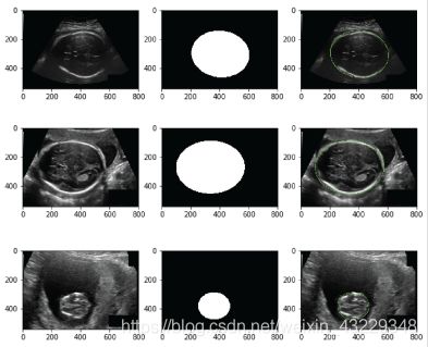
对象边界通常由二进制掩码定义。从二进制掩码中，我们可以通过在图像上覆盖一个轮廓，以勾勒出物体的边界。例如，下面的截图描绘了一个胎儿的超声波图像，一个对应于胎儿头部的二进制掩膜，以及勾勒出在超声波图像上胎儿头部的边界。

其他的例子包括在MRI或CT图像中分割心腔，以计算多个临床指标，包括射血分数。

自动单目标分割的目标是预测给定图像中的二值掩模。在本章中，我们将学习如何创建一个算法来自动分割超声图像中的胎儿头部。这是医学成像中测量胎儿头围的重要任务。

在本章中，我们将介绍以下教程:

• 自定义数据集
• 构建模型
• 定义损失函数与优化器
• 模型训练
• 模型部署

自定义数据集

我们将使用来自 Grand Challenge 网站上胎儿头围自动测量Automated measurement of fetal head circumference比赛的数据。在怀孕期间，超声成像被用来测量胎儿的头围。这种测量可以用来监测胎儿的生长。该数据集包含标准平面的二维超声图像.

在本教程中，我们将使用torch.utils.data包中的Dataset类来创建用于加载和处理数据的自定义数据集。

准备工作

通过以下步骤下载数据集：

• 下载training_set.zip和test_set.zip文件
• 将ZIP文件移动到与代码相同位置的名为data的文件夹中，并将它们分别解压为training_set和test_set。training_set文件夹包含999张.png图片和999个标注文件。test_set文件夹包含335.png图片，没有标注文件。

我们将使用training_set文件夹中的图片和标注文件训练模型。在test_set文件夹上部署模型。

数据探索

我们首先探索数据和显示一些样本以及对应的mask

1. 通过计算图像数目和标注文件数目来检查training_set文件夹

import os
path2train = "./data/training_set/"
imgsList=[pp for pp in os.listdir(path2train) if "Annotation" not in pp]
anntsList=[pp for pp in os.listdir(path2train) if "Annotation" in pp]
print("number of images:", len(imgsList))
print("number of annotations:", len(anntsList))

# number of images: 999
# number of annotations:999

2. 下一步，我们将显示一些样本图像和mask信息

import numpy as np
np.random.seed(2021)
rndImgs=np.random.choice(imgsList,4)
print(rndImgs)
# array(['425_HC.png', '804_HC.png', '603_HC.png', '082_HC.png'], dtype='
# 定义一个辅助函数显示图片和mask
import matplotlib.pylab as plt
from PIL import Image
from scipy import ndimage as ndi
from skimage.segmentation import mark_boundaries

def show_img_mask(img, mask):
	img_mask=mark_boundaries(np.array(img), np.array(mask), outline_color=(0,1,0),color=(0,1,0))
	plt.imshow(img_mask)

# 调用辅助函数显示图片和mask
for fn in rndImgs:
	path2img=os.path.join(path2train, fn)
	path2annt=path2img.replace(".png","_Annotation.png")
	img=Image.open(path2img)
	annt_edges=Image.open(path2annt)
	mask=ndi.binary_fill_holes(annt_edges)
	
	plt.figure()
	plt.subplot(1,3,1)
	plt.imshow(img, cmap="gray")

	plt.subplot(1,3,2)
	plt.imshow(mask,cmap="gray")

	plt.subplot(1,3,3)
	show_img_mask(img, mask)

数据增强

我们将使用albumentations包来增强分割任务的数据：

#1. 安装albumentations包
pip install imgaug
pip install albumentations

#2. 导入数据增强函数
from albumentations import HorizontalFlip, VerticalFlip, Compose, Resize

#3. 为训练集定义transform_train函数
h,w=128,192
transform_train=Compose([Resize(h,w),
						HorizontalFlip(p=0.5),
						VerticalFlip(p=0.5),])
#4. 为验证集定义transform_val函数
transform_val=Resize(h,w)

创建数据集

我们将创建训练数据集和验证集

#1. 导入相应的包以及定义dataset类
from torch.utils.data import Dataset
from PIL import Image
from torchvision.transforms.functional import to_tensor, to_pil_image
# 定义fetal_dataset类
class fetal_dataset(Dataset):
	def __init__(self, path2data, transform=None):
		imgsList=[pp for pp in os.listdir(path2data) if "Annotation" not in pp]
		anntsList=[pp for pp in os.listdir(path2train) if "Annotation" in pp]
		self.path2imgs=[os.path.join(path2data, fn) for fn in imgsList]
		self.path2annts=[p2i.replace(".png","_Annotation.png") for p2i in self.path2imgs]
		self.transform=transform
	
	def __len__(self):
		return len(self.path2imgs)
	
	def __getitem__(self, idx):
		path2img = self.path2imgs[idx]
		image=Image.open(path2img)
		path2annt = self.path2annts[idx]
		mask=ndi.binary_fill_holes(annt_edges)
		image=np.array(image)
		mask=mask.astype("uint8")
		if self.transform:
			augmented=self.transform(image=image, mask=mask)
			image=augmented["image"]
			mask=augmented["mask"]
		image = to_tensor(image)
		mask=255*to_tensor(mask)
		return image, mask
#2. 定义fetal_dataset类的两个实例对象
fetal_ds1=fetal_dataset(path2train, transform=transform_train)
fetal_ds1=fetal_dataset(path2train, transform=transform_val)
print(len(fetal_ds1))
print(len(fetal_ds2))
# 999
# 999

#3. 从feta_ds1中获取一个样本图像和掩码并显示它:
img,mask=fetal_ds1[0]
print(img.shape, img.type(), torch.max(img))
print(mask.shape,mask.type(),torch.max(mask))
# torch.Size([1, 128, 192]) torch.FloatTensor tensor(0.9373)
# torch.Size([1,128,192]) torch.FloatTensor tensor(1.)
show_img_mask(img, mask)

#4. 将数据分为两个部分
from sklearn.model_selection import ShuffleSplit
sss = ShuffleSplit(n_split=1, test_size=0.2, random_state=0)
indices=range(len(fetal_ds1))
for train_index, val_index in sss.split(indices):
	print(len(train_index))
	print("-"*10)
	print(len(val_index))
# 799
# -------
# 200

#5. 创建train_ds和val_ds
from torch.utils.data import Subset
train_ds=Subset(fetal_ds1, train_index)
print(len(train_ds))

val_ds=Subset(fetal_ds2,val_index)
print(len(val_ds))
# 799
# 200
#6. 显示train_ds的一个样例
plt.figure(figsize=(5,5))
for img,mask in train_ds:
	show_img_mask(img,mask)
	break
plt.figure(figsize=(5,5))
for img,mask in val_ds:
	show_img_mask(img,mask)
	break	

#7.定义数据加载器
from torch.utils.data import DataLoader

train_dl = DataLoader(train_ds, batch_size=8, shuffle=True)
val_dl=DataLoader(val_ds,batch_size=16,shuffle=False)

#8.获取train_dl的一小批样例信息
for img_b, mask_b in train_dl:
	print(img_b.shape, img_b.dtype)
	print(mask_b.shape, mask_b.dtype)
	break
# torch.Size([8,1,128,192]) torch.uint8
# torch.Size([8,1,128,192]) torch.uint8

# 获取val_dl的一小批样例信息
for img_b, mask_b in val_dl:
	print(img_b.shape, img_b.dtype)
	print(mask_b.shape, mask_b.dtype)
	break
# torch.Size([16,1,128,192]) torch.uint8
# torch.Size([16,1,128,192]) torch.uint8

代码解析：
在数据探索小节中，我们检查了数据以了解更多关于它的信息。首先，我们在training_set文件夹中获得了图像和标注的列表。标注文件的文件名中有关键字“Annotation”。正如之前所了解的，文件夹中有999张图片和999个标注文件。

在步骤2中，我们显示了一些随机图像和标注。我们定义了一个辅助函数show_img_mask来显示图像和mask。辅助函数的输入如下:

• image: 一张PIL类型的图片
• mask:包含目标的二进制掩码的PIL或numpy数组

在函数中，我们使用了来自skimage.segmentation包里面的mark_boundaries函数在图像上显示目标的轮廓。

注意，标注文件包含胎儿头部的边缘。因此，我们使用scipy.ndimage包中的binary_fill_holes函数将边缘转换为二进制掩码。屏幕截图左边是原始的超声图像，中间是胎儿头部的二进制掩码，右边是图像叠加。

在数据增强小节中，我们使用了一个流行的名为albumentations的Python包来进行数据增强。该包具有一套丰富的各种增强和转换技术。在步骤2中，我们导入了其中几个包。接下来，对于训练数据集，我们使用了一个垂直和水平翻转，将图像大小调整为128 x 192。对于验证数据集，我们只执行了调整大小的转换。

在创建数据集类小节中，我们使用了来自torch.utils.data包的dataset类来创建自定义的训练和验证数据集。在步骤1，我们定义了fetal_dataset类。这个类有三个函数。第一个函数是__init__函数，有三个输入，如下所示:

• self:指向类的指针
• path2data:一个指向数据路径的字符串
• transform:变换函数
  在这个函数中，我们得到了图像和标注的列表，并初始化了变量。

类的第二个函数__len__返回数据集的长度。最后，__getitem__函数加载图像和标注文件，并返回图像和二进制掩码。注意，我们在最后使用to_tensor函数将数组转换为PyTorch张量。to_tensor函数将这些值通过除以255进行归一化。因此，我们通过将掩码值乘以255将其缩小到[0,1]的范围。

在步骤2中，我们通过将transform_train和transform_val分别传递给fetal_dataset类来定义两个对象。正如预期的那样，fetal_ds1和fetal_ds2的长度都是999。

在第3步中，我们从fetal_ds1获取并显示了一个图像和一个掩码。注意图像和掩码中的形状、类型和最大值。正如你所看到的，图片和掩码的大小已经调整为128 x 192，torch.FloatTensor类型，最大值为1。

在第4步中，通过将20%的索引从总索引中分离出来，我们创建了两个train_index和val_index列表。

在第5步中，我们将train_index和val_index从torch.utils.data包传递给Subset类，分别创建训练和验证数据集。

在第6步中，我们分别显示了来自train_ds和val_ds的示例图像和掩码。

在步骤7中，我们定义了两个数据加载器train_dl和val_dl，使用DataLoader类能够在训练期间从训练和验证数据集中获取批数据。

在步骤8中，我们从train_dl和val_dl获得了一批数据，并打印了它们各自的形状。正如我们所看到的，从数据加载器返回了尺寸为[batch_size, 128, 192]的张量。

定义模型

用于分割任务的流行模型架构是所谓的编码器-解码器模型，如下图所示:

在编码器-解码器模型的前半部分，使用几层卷积神经网络(CNNs)和池化层将输入图像缩小为特征图。在模型的第二部分，特征图被上采样到输入图像的大小以产生一个二值掩码。

基于ResNet的跳跃连接的概念，实现了一个流行的编码器-解码器模型架构U-Net。在这个教程中，将学习如何使用PyTorch去实现单目标分割。

#1. 导入必要的包
import torch.nn as nn
import torch.nn.functional as F

class SegNet(nn.Modulo):
	def __init__(self, params):
		super(SegNet, self).__init__()
		C_in, H_in, W_in=params["input_shape"]
		init_f=params["initial_filters"]
		num_outputs=params["num_outputs"]
		self.conv1=nn.Conv2d(C_in, init_f, kernel_size=3, stride=1, padding=1)
		self.conv2=nn.Conv2d(init_f, 2*init_f,kernel_size=3,stride=1,padding=1)
		self.conv3=nn.Conv2d(2*init_f, 4*init_f,kernel_size=3,stride=1,padding=1)
		self.conv4=nn.Conv2d(4*init_f, 8*init_f,kernel_size=3,stride=1,padding=1)
		self.conv5=nn.Conv2d(8*init_f, 16*init_f,kernel_size=3,stride=1,padding=1)
		
		self.upsample=nn.Upsample(scale_factor=2,mode="bilinear",align_corners=True)
		self.conv_up1=nn.Conv2d(16*init_f, 8*init_f, kernel_size=3, stride=1, padding=1)
		self.conv_up2=nn.Conv2d(8*init_f, 4*init_f, kernel_size=3, stride=1, padding=1)
		self.conv_up3=nn.Conv2d(4*init_f, 2*init_f, kernel_size=3, stride=1, padding=1)
		self.conv_up4=nn.Conv2d(2*init_f, 1*init_f, kernel_size=3, stride=1, padding=1)
		self.conv_out=nn.Conv2d(init_f, num_outputs, kernel_size=3, padding=1)
	
	def forward(self, x):
		x = F.relu(self.conv1(x))
		x = F.max_pool2d(x, 2, 2)

		x = F.relu(self.conv2(x))
		x = F.max_pool2d(x, 2, 2)
		
		x = F.relu(self.conv3(x))
		x = F.max_pool2d(x, 2, 2)

		x = F.relu(self.conv4(x))
		x = F.max_pool2d(x, 2, 2)
		
		x = F.relu(self.conv5(x))
		
		x = self.upsample(x)
		x = F.relu(self.conv_up1(x))
		
		x = self.upsample(x)
		x = F.relu(self.conv_up2(x))
		
		x = self.upsample(x)
		x = F.relu(self.conv_up3(x))
		
		x = self.upsample(x)
		x = F.relu(self.conv_up4(x))

		x = self.conv_out(x)
		
#2. 定义SegNet类的一个实例对象
params_model={
	"input_shape":(1,h,w),
	"initial_filters":16,
	"num_outputs":1
	}	
model=SegNet(params_model)
#3. 将模型移到GPU设备上
import torch
device = torch.device("cuda" if torch.cuda.is_available() else "cpu")
nodel=model.to(device)

#4. 打印模型
print(model)
# SegNet(
# (conv1): Conv2d(1, 16, kernel_size=(3, 3), stride=(1, 1), padding=(1, 1))
# (conv2): Conv2d(16, 32, kernel_size=(3, 3), stride=(1, 1),padding=(1, 1))
# (conv3): Conv2d(32, 64, kernel_size=(3, 3), stride=(1, 1),padding=(1, 1))
# (conv4): Conv2d(64, 128, kernel_size=(3, 3), stride=(1, 1),padding=(1, 1))
# (conv5): Conv2d(128, 256, kernel_size=(3, 3), stride=(1, 1),padding=(1, 1))
# (upsample): Upsample(scale_factor=2.0, mode=bilinear)
# (conv_up1): Conv2d(256, 128, kernel_size=(3, 3), stride=(1, 1),padding=(1, 1))
# (conv_up2): Conv2d(128, 64, kernel_size=(3, 3), stride=(1, 1),padding=(1, 1))
# (conv_up3): Conv2d(64, 32, kernel_size=(3, 3), stride=(1, 1),padding=(1, 1))
# (conv_up4): Conv2d(32, 16, kernel_size=(3, 3), stride=(1, 1),padding=(1, 1))
# (conv_out): Conv2d(16, 1, kernel_size=(3, 3), stride=(1, 1),padding=(1, 1))
# )

#5. 显示模型概要
from torchsummary import summary
summary(model, input_size=(1, h, w), device=device.type)
#----------------------------------------------------------------
# Layer (type)         Output Shape               Param #
# ================================================================
# Conv2d-1         [-1, 16, 128, 192]             160
# Conv2d-2         [-1, 32, 64, 96]             4,640
# Conv2d-3         [-1, 64, 32, 48]            18,496
# Conv2d-4         [-1, 128, 16, 24]           73,856
# Conv2d-5         [-1, 256, 8, 12]           295,168
# Upsample-6       [-1, 256, 16, 24]                0
# Conv2d-7         [-1, 128, 16, 24]          295,040
# Upsample-8       [-1, 128, 32, 48]                0 		
# Conv2d-9         [-1, 64, 32, 48]            73,792
# Upsample-10      [-1, 64, 64, 96]                 0
# Conv2d-11        [-1, 32, 64, 96]            18,464
# Upsample-12      [-1, 32, 128, 192]               0
# Conv2d-13        [-1, 16, 128, 192]           4,624
# Conv2d-14        [-1, 1, 128, 192]              145
# ================================================================	

代码解析
在步骤1中，我们定义了模型类SegNet。我们首先导入所需的包。模型类是由__init__和forward函数构建的。这个函数的输入是一个包含模型参数的Python字典:

• params:包含模型参数的Python字典
  字典的关键字如下：
• input_shape:一个元组，模型输入形状(1,height,width)
• initial_filters:一个整数，表示第一个CNN层的卷积核个数
• num_outputs:一个整数，输出通道数目；传入1表示单目标分割

在__init__函数中，我们定义了模型的构建块。这包括五个CNN块用于向下采样输入，一个向上采样块，另外五个CNN块用于向上采样feature map。

在forward函数中，我们定义了层与层之间的连接。forward函数的输入是一个具有(batch_size, 1, height, width)形状的张量。正如我们所见，输入图像经过CNN和max-pooling块，然后被上采样到输入图像的大小。

注意，模型定义中的输出层没有应用激活函数。

在步骤2中，我们定义了一个SegNet类的对象，并将其称为model。在步骤3中，如果GPU设备可用，我们将模型移动到该设备上。在步骤4中，我们打印了模型。在步骤5中，我们使用torchsummary包打印模型摘要。

定义损失函数和优化器

到目前为止，我们已经创建了一个数据集和一个模型。为了训练模型，我们需要定义一个损失函数和一个优化器来根据损失的梯度更新模型参数。经典的单目标分割损失函数是二元交叉熵(BCE)损失函数。BCE损失函数将预测的每个像素与真实值进行比较;然而，我们可以结合多个标准来提高分割任务的整体性能。一种流行的技术是将dic度量与BCE损失相结合。dic度量通过计算真实和预测之间的重叠量来测试分割算法的性能。在本节中，您将学习如何开发组合损失函数。然后，您将定义优化器，以在训练期间自动更新模型参数。

# 我们将开发联合损失函数，优化器以及学习率策略

# 1.定义一个计算dice度量的辅助函数
def dic_loss(pred, target, smooth=1e-5):
	intersection = (pred * target).sum(dim=(2,3))
	union=pred.sum(dim=(2,3)) + target.sum(dim=(2,3))
	dice=2.0*(intersection + smooth)/(union+smooth)
	loss = 1.0-dice
	return loss.sum(), dice.sum()
#2. 定义一个计算每批次数据的联合损失的辅助函数
import torch.nn.functional as F
def loss_func(pred, target):
	bce=F.binary_cross_entropy_with_logits(pred, target, reduction="sum")
	pred=torch.sigmoid(pred)
	dlv,_=dice_loss(pred, target)
	loss = bce+dlv
	return loss

#3. 定义metrics_batch辅助函数
def metrics_batch(pred, target):
	pred=torch.sigmoid(pred)
	_,metric=dic_loss(pred, target)
	return metric
#4. 定义loss_batch辅助函数
def loss_batch(loss_func, output, target, opt=None):
	loss = loss_func(output, target)
	with torch.no_grad():
		metric_b=metrics_batch(output, target)
	if opt is not None:
		opt.zero_grad()
		loss.backward()
		opt.step()
	return loss.item(), metric_b
#5. 定义优化器
from torch import optim
opt=optim.Adam(model.parameters(),lr=3e-4)
#6. 定义学习率策略
from torch.optim.lr_scheduler import ReduceLROnPlateau
lr_scheduler=ReduceLROnPlateau(opt, mode="min", factor=0.5, patience=20, verbose=1)
def get_lr(opt):
	for param_group in opt.param_groups:
		return param_group["lr"]
current_lr=get_lr(opt)
print("current lr={}".format(current_lr))

代码解析：
在步骤1中，我们定义了dice_loss辅助函数来计算dice损失值。函数的输入如下:

• pred：预测结果，尺寸为(batch_size, 1, height, width)的tensor
• target: 真实值，尺寸为(batch_size,1,height,width)的tensor

函数计算每批次的dice值。dice值在[0，1]之间，其中1表示预测值与真实值完全的重叠。dice loss通过1-dice计算得来。函数最终返回每批次的损失值之和。

在步骤2中，我们定义了loss_func辅助函数来计算每个批数据的组合损失值。该函数有两个输入:

• pred:形状为(batch_size, 1, height, width)的预测值张量
• target:形状为(batch_size,1,height,width)的真实值张量

函数中，首先计算二元交叉熵损失，然后计算dice loss，并且返回每批次的两种损失之和。

注意，sigmoid操作集成到binary_cross_entropy_with_logits函数中。记住，模型输出不包括sigmoid激活函数。

在第3步中，我们定义了metrics_batch辅助函数来为每个批处理计算一个度量指标。您可以在这个辅助函数中计算任何度量。我们通过调用dice_loss辅助函数来计算dice度量。dice度量是评估分割任务的流行度量。

在第4步中，我们定义了loss_batch 辅助函数。辅助函数的输入如下:

• loss_func:第二步中的联合损失函数
• output:预测值，形状为(batch_size, 1, height, width)
• target:真实值,形状为(batch_size, 1, height,width)
• opt:优化器对象

在函数中，我们计算每批次数据的损失和度量值。在训练期间，优化器对象被传递给辅助函数，使用opt.step()更新模型参数。

在步骤5中，我们定义了Adam优化器来在训练期间优化模型。

在步骤6中，我们定义了学习率计划，在训练过程中，在满足patience=20的情况下，自动降低学习率。

模型训练

到目前为止，我们已经学习了如何创建训练和验证数据集，建立模型，并定义损失函数和优化器。现在，是时候训练模型了。这是一个迭代过程。在每次迭代中，我们从训练数据集中选择一批数据。然后我们将数据提供给模型以获得模型输出。然后，我们计算损失值。接下来，我们计算损失函数相对于模型参数的梯度(也称为权重)。最后，优化器根据梯度更新参数，然后继续这个循环。我们还使用验证数据集在训练期间监控模型性能。当表现趋于稳定时，我们将停止训练过程。为了提高代码的可读性，我们将定义一些辅助函数。

#1. 定义loss_epoch辅助函数
def loss_epoch(model, loss_func, dataset_dl, sanity_check=False, opt=None):
	running_loss=0.0
	running_metric=0.0
	len_data = len(dataset_dl.dataset)
	for xb, yb in dataset_dl:
		xb=xb.unsqueeze(1).type(torch.float32).to(device)
		yb=yb.unsqueeze(1).type(torch.float32).to(device)
		output=model(xb)
		loss_b, metric_b=loss_batch(loss_func, output, yb, opt)
		running_loss += loss_b

		if metric_b is not None:
			running_metric += metric_b
		if sanity_check is True:
			break
	loss = running_loss/float(len_data)
	metric=running_metric/float(len_data)
	return loss, metric

#2. 定义train_val辅助函数
import copy
def train_val(model, params):
	num_epochs=params["num_epochs"]
	loss_func=params["loss_func"]
	opt=params["optimizer"]
	train_dl=params["train_dl"]
	val_dl=params["val_dl"]
	sanity_check=params["sanity_check"]
	lr_scheduler=params["lr_scheduler"]
	path2weights=params["path2weights"]
	loss_history={
	"train":[],
	"val":[]
	}
	metric_history={
	"train":[],
	"val":[]
	}
	best_model_wts=copy.deepcopy(model.state_dict())
	best_loss=float("inf")
	for epoch in range(num_epochs):
		current_lr=get_lr(opt)
		print("Epoch {}/{}, current lr={}".format(epoch, num_epochs-1, current_lr))
		model.train()
		train_loss,train_metric=loss_epoch(model,loss_func,train_dl,sanity_check,opt)
		loss_history["train"].append(train_loss)
		metric_history["train"].append(train_metric)
		model.eval()
		with torch.no_grad():
			val_loss, val_metric=loss_epoch(model, loss_func, val_dl, sanity_check)
		loss_history["val"].append(val_loss)
		metric_history["val"].append(val_metric)
		if val_loss < best_loss:
			best_loss=val_loss
			best_model_wts=copy.deepcopy(model.state_dict())
			torch.save(model.state_dict(), path2weights)
			print("Copied best model weights!")
		lr_scheduler.step(val_loss)
		if current_lr != get_lr(opt):
			print("Loading best model weights")
			model.load_state_dict(best_model_wts)
		print("train loss: %.6f, dice: %.2f" % (train_loss, 100*train_metric)
		print("val loss: %.6f, dice: %.2f" % (val_loss, 100*val_metric)
		print("-"*10)
	model.load_state_dict(best_model_wts)
	return model, loss_history, metric_history
#3. 调用train_val函数训练模型
path2models="./models/"
if not os.path.exists(path2models):
	os.mkdir(path2models)
params_train={
	"num_epochs":100,
	"optimizer":opt,
	"loss_func":loss_func,
	"train_dl":train_dl,
	"val_dl":val_dl,
	"sanity_check":False,
	"lr_scheduler":lr_scheduler,
	"path2weights":path2models+"weights.pt",
}			
model,loss_hist,metric_hist=train_val(model,params_train)

# Epoch 0/99, current lr=0.0003
# Copied best model weights!
# train loss: 8438.457021, accuracy: 61.10
# val loss: 4836.094668, accuracy: 79.14
# ----------
# Epoch 1/99, current lr=0.0003
# Copied best model weights!
# train loss: 4296.525105, accuracy: 78.74
# val loss: 4189.101631, accuracy: 82.83
# ...


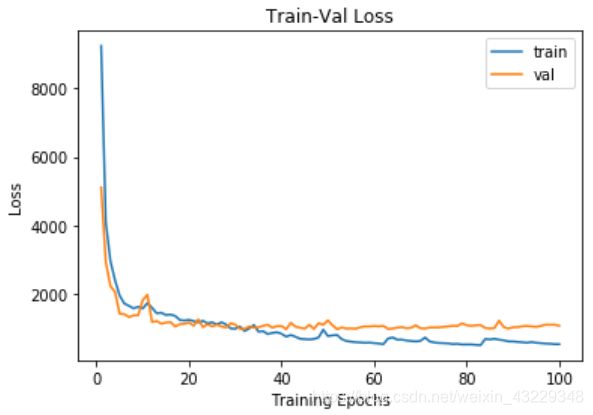
#4. 让我们绘制出训练和验证损失的过程
num_epochs=params_train["num_epochs"]
plt.title("Train-Val Loss")
plt.plot(range(1,num_epochs+1),loss_hist["train"], label="train")
plt.plot(range(1, num_epochs+1), loss_hist["val"], label="val")
plt.ylabel("Loss")
plt.xlabel("Training Epochs")
plt.legend()
plt.show()

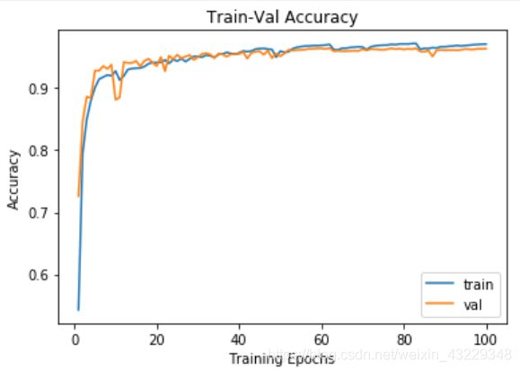
# 绘制出dice
plt.title("Train-Val Accuracy")
plt.plot(range(1,num_epochs+1), metric_hist["train"], label="train")
plt.plot(range(1,num_epochs+1),metric_hist["val"],label="val")
plt.ylabel("Accuracy")
plt.xlabel("Training Epochs"]
plt.legend()
plt.show()

代码解析：
在步骤1中，我们定义了loss_epoch辅助函数。函数输入如下:

• model:模型对象
• loss_func:损失函数对象
• dataset_dl:数据加载器对象
• sanity_check:默认是False
• opt:优化器对象

在函数中，我们从数据加载器中提取批数据，xb和yb张量。接下来，我们得到模型输出，并计算每批数据的损失和度量值。我们对整个数据集重复此过程，并返回平均损失和度量值。

在步骤2中，我们定义了train_val辅助函数。函数的输入如下:

• model:模型对象
• params:包含训练参数的Python字典

在函数中，我们对模型进行num_epochs次迭代训练。在每次迭代中，我们将模型设置为train模式，并对模型进行一个epoch的训练。然后在验证数据集上对模型进行评估。如果验证结果在每次迭代中得到改进，我们存储模型参数。如果验证性能在patience次内不改善，根据学习率策略，降低学习率。该函数返回训练好的模型和包含每次迭代的损失值和度量值的两个字典。

在第3步中，我们在params_train中设置训练参数，并调用train_val函数来训练模型。

在步骤4中，我们绘制了训练结果和验证损失值，以查看多个epoch的训练过程。

部署模型

一旦训练完成，您将希望将模型部署到新数据上。在本教程中，您将学习如何在test_set数据集上部署模型。我们将假设您想要在一个新的脚本中部署用于推理的模型，而不是训练脚本。在这种情况下，模型在内存中不存在。为了避免重复，我们将跳过模型定义。在执行以下步骤之前，请确保您在部署代码中按照定义模型部分的解释定义了模型。

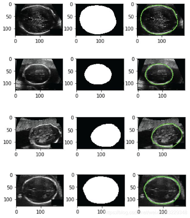
我们将从test_set数据集中加载一些图像，将它们提供给经过训练的模型，然后显示输出:

#1. 获取test_set路径下的图像列表
import os
path2test="./data/test_set/"
imgsList=[pp for pp in os.listdir(path2test) if "Annotation" not in pp]
print("number of images:", len(imgsList))
# number of images: 335

#2. 随机采样
import numpy as np
np.random.seed(2019)
rndImgs=np.random.choice(imgsList,4)
print(rndImgs)
# array(['043_HC.png', '011_HC.png', '303_HC.png', '091_HC.png'], dtype='

#3.构建模型
import torch.nn as nn
import torch.nn.functional as F
class SegNet(nn.Module):
	def __init__(self, params):
		super(SegNet, self).__init__()
		C_in, H_in, W_in = params["input_shape"]
		init_f=params["initial_filters"]
		num_outputs=params["num_outputs"]
		self.conv1 = nn.Conv2d(C_in, init_f, kernel_size=3,stride=1,padding=1)
        self.conv2 = nn.Conv2d(init_f, 2*init_f, kernel_size=3,stride=1,padding=1)
        self.conv3 = nn.Conv2d(2*init_f, 4*init_f, kernel_size=3,padding=1)
        self.conv4 = nn.Conv2d(4*init_f, 8*init_f, kernel_size=3,padding=1)
        self.conv5 = nn.Conv2d(8*init_f, 16*init_f, kernel_size=3,padding=1)

        self.upsample = nn.Upsample(scale_factor=2, mode='bilinear', align_corners=True)

        self.conv_up1 = nn.Conv2d(16*init_f, 8*init_f, kernel_size=3,padding=1)
        self.conv_up2 = nn.Conv2d(8*init_f, 4*init_f, kernel_size=3,padding=1)
        self.conv_up3 = nn.Conv2d(4*init_f, 2*init_f, kernel_size=3,padding=1)
        self.conv_up4 = nn.Conv2d(2*init_f, init_f, kernel_size=3,padding=1)

        self.conv_out = nn.Conv2d(init_f, num_outputs , kernel_size=3,padding=1)
    
		    
    def forward(self, x):
        
        x = F.relu(self.conv1(x))
        x = F.max_pool2d(x, 2, 2)

        x = F.relu(self.conv2(x))
        x = F.max_pool2d(x, 2, 2)

        x = F.relu(self.conv3(x))
        x = F.max_pool2d(x, 2, 2)

        x = F.relu(self.conv4(x))
        x = F.max_pool2d(x, 2, 2)

        x = F.relu(self.conv5(x))

        x=self.upsample(x)
        x = F.relu(self.conv_up1(x))

        x=self.upsample(x)
        x = F.relu(self.conv_up2(x))
        
        x=self.upsample(x)
        x = F.relu(self.conv_up3(x))
        
        x=self.upsample(x)
        x = F.relu(self.conv_up4(x))

        x = self.conv_out(x)
        
        return x

#4. 模型初始化
h,w=128,192
params_model={
        "input_shape": (1,h,w),
        "initial_filters": 16, 
        "num_outputs": 1,
            }

model = SegNet(params_model)
#5. 将模型移到GPU设备上
import torch
device = torch.device('cuda:1' if torch.cuda.is_available() else 'cpu')
model=model.to(device)


#6.显示辅助函数
import matplotlib.pylab as plt
from PIL import Image
from scipy import ndimage as ndi
from skimage.segmentation import mark_boundaries

def show_img_mask(img, mask):
    
    img_mask=mark_boundaries(np.array(img), 
                        np.array(mask),
                        outline_color=(0,1,0),
                        color=(0,1,0))
    plt.imshow(img_mask)

#7. 导入训练好的模型权重
path2weights="./models/weights.pt"
model.load_state_dict(torch.load(path2weights))
model.eval()

#8. 导入图片，并输入到模型中
from torchvision.transforms.functional import to_tensor, to_pil_image
for fn in rndImgs:
	path2img = os.path.join(path2train, fn)
	img = Image.open(path2img)
	img = img.resize((w, h))
	img_t = to_tensor(img).unsqueeze(0).to(device)
	pred = model(img_t)
	pred = torch.sigmoid(pred)[0]
	mask_pred = (pred[0]>=0.5)
	plt.figure()
	plt.subplot(1,3,1)
	plt.imshow(img, cmap="gray")
	plt.subplot(1,3,2)
	plt.imshow(mask_pred, cmap="gray")
	plt.subplot(1,3,3)
	show_img_mask(img,mask_pred)

代码解析：
在步骤1中，我们在test_set文件夹中获得了图像列表。正如你看到的，有335张图像，测试集没有标注文件。

在步骤2中，我们随机选取了4张图像。
在步骤3中，构建SegNet模型
在步骤4中，初始化模型结构
在步骤5中，将模型移到GPU设备上
在步骤6中，显示辅助函数
在步骤7中，导入训练好的模型权重，model.eval()方法将模型建立在评估模式下。
在步骤8中，我们逐个加载图像，并将它们提供给模型。在向模型输入图像之前，我们将其大小调整为(128,192)，并将其转换为PyTorch张量。然后将模型输出传递给sigmoid激活函数，并与0.5阈值进行比较，得到二进制掩码。接下来，我们显示图像，预测得到的目标二值掩模，并在图像上画出目标的轮廓。正如你所看到的，该模型能够在超声波图像中准确地检测胎儿头部。