DS Wannabe之5-AM Project: DS 30day int prep day7

Q1. What is the process to make data stationery from non- stationary in time series?

The two most common ways to make a non-stationary time series stationary are:

• Differencing
• Transforming

Let us look at some details for each of them:

Differencing

X1, X2, X3,...........Xn

Your series with a difference of degree 1 becomes:

(X2 - X1, X3 - X2, X4 - X3,.......Xn - X(n-1)

To make your series stationary, you take a difference between the data points. So let us say, your original time series was:

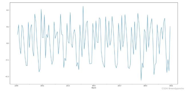
Once, you make the difference, plot the series and see if there is any improvement in the ACF curve. If not, you can try a second or even a third-order differencing. Remember, the more you difference, the more complicated your analysis is becoming.

将非平稳时间序列转换为平稳序列的两种常见方法是差分和变换。差分是通过计算连续数据点之间的差值来实现的。例如，原始时间序列为X1, X2, X3,...,Xn，一阶差分后的序列为(X2 - X1, X3 - X2, X4 - X3,...,Xn - X(n-1))。如果差分后的序列仍不平稳，可以尝试二阶或三阶差分。差分次数越多，分析过程越复杂。差分后，应绘制序列图并检查自相关函数（ACF）曲线是否有所改善。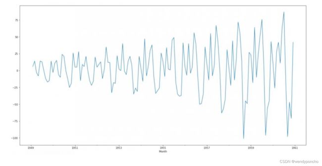

Transforming

If we cannot make a time series stationary, you can try out transforming the variables. Log transform is probably the most commonly used transformation if we see the diverging time series. However, it is suggested that you use transformation only in case differencing is not working.

Q2. What is the process to check stationary data ?

Stationary series: It is one in which the properties – mean, variance and covariance, do not vary

with time.

Let us get an idea with these three plots:

• In the first plot, we can see that the mean varies (increases) with time, which results in an upward trend. This is the non-stationary series. For the series classification as stationary, it should not exhibit the trend.
• Moving on to the second plot, we do not see a trend in the series, but the variance of the series is a function of time. As mentioned previously, a stationary series must have a constant variance
• If we look at the third plot, the spread becomes closer, as the time increases, which implies that covariance is a function of time.

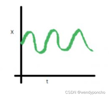
These three plots refer to the non-stationary time series. Now give your attention to fourth:

In this case, Mean, Variance and Covariance are constant with time. This is how a stationary time series looks like.

Most of the statistical models require the series to be stationary to make an effective and precise prediction. The various process you can use to find out your data is stationary or not by the following terms:

1. Visual Test
2. Statistical Test
3. ADF(Augmented Dickey-Fuller) Test
4. KPSS(Kwiatkowski-Phillips-Schmidt-Shin) Test

Q3. What are ACF and PACF?

ACF is a (complete) auto-correlation function which gives us the values of the auto-correlation of any series with lagged values. We plot these values along with a confidence band.We have an ACF plot. In simple terms, it describes how well the present value of the series is related to its past values. A time series can have components like the trend, seasonality, cyclic and residual. ACF considers all the components while finding correlations; hence, it’s a ‘complete auto-correlation

PACF is a partial autocorrelation function. Instead of finding correlations of present with lags like ACF, it finds the correlations of the residuals with the next lag value thus ‘partial’ and not ‘complete’ as we remove already found variations before we find next correlation. So if there are any hidden pieces of information in the residual which can be modelled by next lag, we might get a good correlation, and we’ll keep that next lag as a feature while modelling. Remember, while  modelling we don’t want to keep too many correlated features, as that it can create multicollinearity issues. Hence we need to retain only relevant features.

要检查数据是否平稳，可以通过观察数据的统计特性（如均值、方差和协方差）随时间的变化情况来进行。平稳序列的这些特性不随时间变化。可以通过视觉检查（如绘制时间序列图）和统计检验（如ADF检验和KPSS检验）来确定数据是否平稳。ACF（自相关函数）和PACF（偏自相关函数）图也是分析时间序列数据中自相关性的有用工具，有助于识别数据中的模式和结构。

Q4. What do you understand by the trend of data?

A general systematic linear or (most often) nonlinear component that changes over time and does not repeat.

There are different approaches to understanding trend. A positive trend means it is likely that growth continues. Let's illustrate this with a simple example: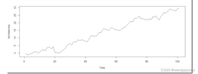

Hmm, this looks like there is a trend. To build up confidence, let's add a linear regression for this graph: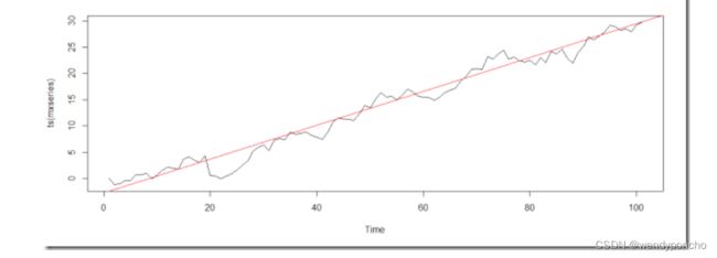

Great, now it’s clear theirs a trend in the graph by adding Linear Regression.

Q5. What is the Augmented Dickey-Fuller Test?

The Dickey-Fuller test: It is one of the most popular statistical tests. It is used to determine the presence of unit root in a series, and hence help us to understand if the series is stationary or not.

The null and alternate hypothesis for this test is:

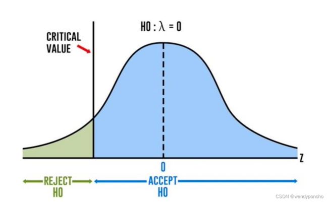
Null Hypothesis: The series has a unit root (value of a =1)

Alternate Hypothesis: The series has no unit root.

If we fail to reject the null hypothesis, we can say that the series is non-stationary. This means that the series can be linear or difference stationary.

Dickey-Fuller增强型检验是一种统计检验，用于检查时间序列中是否存在单位根，从而帮助我们判断序列是否平稳。该检验的原假设是序列有单位根（即非平稳），备择假设是序列没有单位根（即平稳）。

AIC（赤池信息准则）和BIC（贝叶斯信息准则）是时间序列分析中用来评估模型拟合优度的指标，它们通过考虑模型复杂度（参数数量）和数据拟合程度来帮助选择最佳模型。

Q6. What is AIC and BIC into time series?

Akaike’s information criterion (AIC) compares the quality of a set of statistical models to each other. For example, you might be interested in what variables contribute to low socioeconomic status and how the variables contribute to that status. Let’s say you create several regression models for various factors like education, family size, or disability status; The AIC will take each model and rank them from best to worst. The “best” model will be the one that neither under-fits nor over-fits.

Q7. What are the components of the Time -Series?

Time series analysis: It provides a body of techniques to understand a dataset better. The most useful one is the decomposition of the time series into four constituent parts

1. Level- The baseline value for the series if it were a straight line.
2. Trend - The optional and linear, increasing or decreasing behaviour of series over time.
3. Seasonality - Optional repeated patterns /cycles of behaviour over time.
4. Noise - The optional variability in the observations that cannot be explained by the model.

Q8. What is Time Series Analysis? Ans:

Time series analysis: It involves developing models that best capture or describe an observed time series to understand the underlying cause. This study seeks the “why” behind the time-series datasets. This involves making assumptions about the form of data and decomposing time-series into the constitution component.

Quality of descriptive model is determined by how well it describes all available data and the interpretation it provides to inform the problem domain better.

Q9. Give some examples of the Time-Series forecast? 

There is almost an endless supply of the time series forecasting problems. Below are ten examples from a range of industries to make the notions of time series analysis and forecasting more concrete.

1. Forecasting the corn yield in tons by the state each year.

2. Forecasting whether an EEG trace in seconds indicates a patient is having a seizure or not.

3. Forecasting the closing price of stocks every day.

4. Forecasting the birth rates at all hospitals in the city every year.

1. Forecastingproductsalesintheunitssoldeachdayforthestore.

2. Forecastingthenumberofpassengersthroughthetrainstationeachday.

3. Forecasting unemployment for a state each quarter.

4. Forecastingtheutilisationdemandontheservereveryhour.

5. Forecasting the size of the rabbit populations in the state each breeding season.

6. Forecasting the average price of gasoline in a city each day.

Q10. What are the techniques of Forecasting?

Ans:

There are so many statistical techniques available for time series forecast however we have found a few effective ones which are listed below:

• Simple Moving Average (SMA)

• Exponential Smoothing (SES) 

• Autoregressive Integration Moving Average (ARIMA)

Q11. What is the Moving Average? 

The moving average model is probably the most naive approach to time series modelling. This model  states that the next observation is the mean of all past observations.

Although simple, this model might be surprisingly good, and it represents a good starting point.

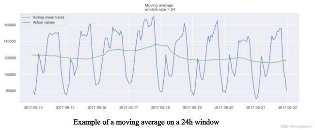
Otherwise, the moving average can be used to identify interesting trends in the data. We can define a window to apply the moving average model to smooth the time series and highlight different trends.

In the plot above, we applied the moving average model to a 24h window. The green line smoothed the time series, and we can see that there are two peaks in the 24h period. The longer the window, the smoother the trend will be.
Below is an example of moving average on a smaller window.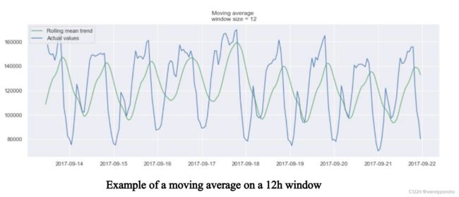

Q12. What is Exponential smoothing?

Exponential smoothing uses similar logic to moving average, but this time, different decreasing weight is assigned to each observation. We can also say, less importance is given to the observations as we move further from the present.

Mathematically, exponential smoothing is expressed as:

Here, alpha is the smoothing factor which takes values between 0 to 1. It determines how fast the weight will decrease for the previous observations.

From the above plot, the dark blue line represents the exponential smoothing of the time series using a smoothing factor of 0.3, and the orange line uses a smoothing factor of 0.05. As we can see, the smaller the smoothing factor, the smoother the time series will be. Because as smoothing factor approaches 0, we approach to the moving average model