基于LightGBM的回归任务案例

在本文中，我们将学习先进的机器学习模型之一：Lightgbm。在对XGB模型进行了越来越多的改进以获得更好的性能之后，XGBoost是一种极限梯度提升机器，但通过lightgbm，我们可以在没有太多计算的情况下实现类似或更好的结果，并在更短的时间内在更大的数据集上训练我们的模型。让我们看看什么是LightGBM以及如何使用LightGBM执行回归。

什么是LightGBM？

LightGBM或“Light Gradient Boosting Machine”是一个开源的高性能梯度增强框架，专为高效和可扩展的机器学习任务而设计。它专门针对速度和准确性而定制，使其成为不同领域中结构化和非结构化数据的热门选择。

LightGBM的关键特性包括它能够处理具有数百万行和列的大型数据集，支持并行和分布式计算，以及优化的梯度提升算法。LightGBM以其出色的速度和低内存消耗而闻名，这要归功于基于直方图的技术和逐叶树生长。

LightGBM如何工作？

LightGBM创建了一个决策树，该决策树按叶子进行开发，这意味着给定一个条件，根据收益只分裂一个叶子。有时候，尤其是对于较小的数据集，叶子树可能会过拟合。可以通过限制树的深度来防止过拟合。LightGBM使用分布的直方图将数据存储到bin中。而不是使用每个数据点，bin用于采样，计算增益，并划分数据。此外，稀疏数据集可以从这种方法的优化中受益。排他性特征捆绑，指的是算法的排他性特征的组合，以减少降维和加速处理，是LightGBM的另一个元素。

还有另一种lightGBM算法用于对数据集进行采样，即，GOSS（基于一致性的单侧采样）。当GOSS计算增益时，具有更大梯度的数据点被赋予更大的权重。为了保持精度，具有较小梯度的数据点被任意删除，而一些保留。在与随机抽样相同的抽样率下，这种方法通常更优越上级。

LightBGM的实现

在本文中，我们将使用这个数据集来执行一个使用lightGBM算法的回归任务。但是要使用LightGBM模型，我们首先必须使用下面的命令安装lightGBM模型：

!pip install lightgbm

Python库使我们能够非常容易地处理数据，并通过一行代码执行典型和复杂的任务。

• Pandas -此库有助于以2D数组格式加载数据框，并具有多个功能，可以一次性执行分析任务。
• Numpy - Numpy数组非常快，可以在很短的时间内执行大型计算。
• Matplotlib/Seaborn -此库用于绘制可视化。
• Sklearn -该模块包含多个库，这些库具有预实现的功能，可以执行从数据预处理到模型开发和评估的任务。

#importing libraries 
import pandas as pd
import numpy as np
import seaborn as sb
import matplotlib.pyplot as plt
import lightgbm as lgb

from sklearn.preprocessing import StandardScaler
from sklearn.model_selection import train_test_split

import warnings
warnings.filterwarnings('ignore')

加载数据集

# Read the data from a CSV file named 'medical_cost.csv' into a DataFrame 'df'.
df = pd.read_csv('medical_cost.csv')
 
# Display the first few rows of the DataFrame to provide a data preview.
df.head()

输出

   Id  age     sex     bmi  children smoker     region      charges
0   1   19  female  27.900         0    yes  southwest  16884.92400
1   2   18    male  33.770         1     no  southeast   1725.55230
2   3   28    male  33.000         3     no  southeast   4449.46200
3   4   33    male  22.705         0     no  northwest  21984.47061
4   5   32    male  28.880         0     no  northwest   3866.85520

df.info()

输出

<class 'pandas.core.frame.DataFrame'>
RangeIndex: 1338 entries, 0 to 1337
Data columns (total 8 columns):
 #   Column    Non-Null Count  Dtype  
---  ------    --------------  -----  
 0   Id        1338 non-null   int64  
 1   age       1338 non-null   int64  
 2   sex       1338 non-null   object 
 3   bmi       1338 non-null   float64
 4   children  1338 non-null   int64  
 5   smoker    1338 non-null   object 
 6   region    1338 non-null   object 
 7   charges   1338 non-null   float64
dtypes: float64(2), int64(3), object(3)
memory usage: 83.8+ KB

#describing the data
print(df.describe())

输出

                Id          age          bmi     children       charges
count  1338.000000  1338.000000  1338.000000  1338.000000   1338.000000
mean    669.500000    39.207025    30.663397     1.094918  13270.422265
std     386.391641    14.049960     6.098187     1.205493  12110.011237
min       1.000000    18.000000    15.960000     0.000000   1121.873900
25%     335.250000    27.000000    26.296250     0.000000   4740.287150
50%     669.500000    39.000000    30.400000     1.000000   9382.033000
75%    1003.750000    51.000000    34.693750     2.000000  16639.912515
max    1338.000000    64.000000    53.130000     5.000000  63770.428010

探索性数据分析

EDA是一种使用可视化技术分析数据的方法。它用于发现趋势和模式，或在统计摘要和图形表示的帮助下检查假设。在执行该数据集的EDA时，我们将尝试查看独立特征之间的关系，即一个特征如何影响另一个特征。

# Define a list of columns to analyze
sample = ['sex', 'children', 'smoker', 'region']

# Iterate through the specified columns
for i, col in enumerate(sample):
	# Group the DataFrame by the current column and calculate the mean of 'charges'
	grouped_data = df[[col, 'charges']].groupby(col).mean()
	
	# Print the mean charges for each group within the current column
	print(grouped_data)
	
	# Print a blank line to separate the output for different columns
	print()

输出

              charges
sex                 
female  12569.578844
male    13956.751178
               charges
children              
0         12365.975602
1         12731.171832
2         15073.563734
3         15355.318367
4         13850.656311
5          8786.035247
             charges
smoker              
no       8434.268298
yes     32050.231832
                charges
region                 
northeast  13406.384516
northwest  12417.575374
southeast  14735.411438
southwest  12346.937377

在这里，这段代码检查显示为DataFrame（‘df’）的医疗费用信息的数据集。最受重视的类别是“性别”、“儿童”、“吸烟者”和“地区”。每一类别的平均医疗费用是在系统地按这些列对数据进行分组后通过算法计算的。输出提供了关于这些分类变量如何影响典型医疗费用的信息。在列之间使用空白行可以提高阅读和理解能力，并允许对数据集的属性进行更全面的解释。从以上结果我们可以得出一些结论。

• 男性的医疗保险费用比女性高。
• 在儿童人数与收费之间没有这种趋势。
• 吸烟者必须支付明显高于非吸烟者的医疗保险费用，因为吸烟者必须面对的健康问题。
• 医疗费用在东南地区最高，西南地区最低，但差别并不大。

分类可视化

# Set the figure size for the subplots
plt.subplots(figsize=(15, 15))

# Define the list of columns to visualize
sample = ['sex', 'children', 'smoker', 'region']

# Loop through the specified columns
for i, col in enumerate(sample):
	# Create subplots in a 3x2 grid
	plt.subplot(3, 2, i + 1)
	
	# Create a countplot for the current column
	sb.countplot(data=df, x=col)
	
# Adjust subplot layout for better presentation
plt.tight_layout()

# Display the subplots
plt.show()

输出

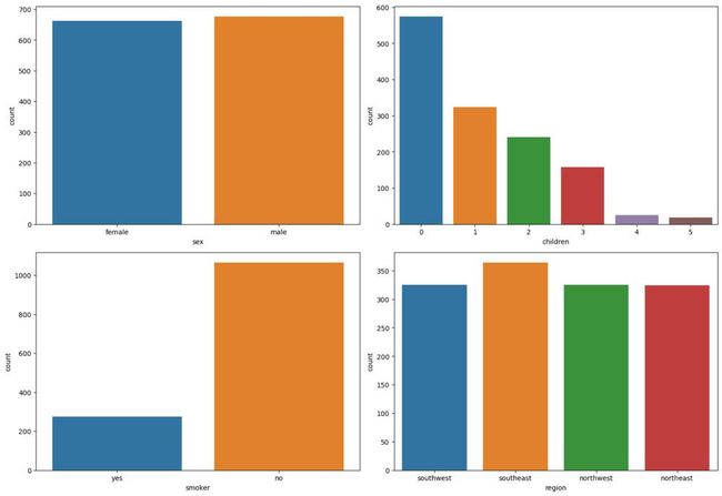
这段代码创建一个子图网格，具有预定的图形大小（3行和2列）。下一步迭代分类列的列表（如“sex”、“children”、“smoker”和“region”）;对于每一列，它生成一个countplot，显示DataFrame（缩写为“df”）中值的分布。最后，子图使用“plt.show（X）”表示，给出数据集中分类数据分布的可视化摘要。'plt.tight_layout（）'函数用于改进子图的布局，以便更好地呈现。从上面的输出，我们可以得出以下几点：

• 数据集中男性和女性的病例数量相等。收集这一数据的四个区域的情况也类似。
• 在数据集中，吸烟者比不吸烟者少。
• 无子女至有5个子女的人数按递减顺序排列。

数字列的分布分析

# Set the figure size for the subplots
plt.subplots(figsize=(15, 15))

# Define the list of numeric columns to visualize
sample = ['age', 'bmi', 'charges']

# Loop through the specified columns
for i, col in enumerate(sample):
	# Create subplots in a 3x2 grid
	plt.subplot(3, 2, i + 1)
	
	# Create a distribution plot for the current numeric column
	sb.distplot(df[col])
	
# Adjust subplot layout for better presentation
plt.tight_layout()

# Display the subplots
plt.show()

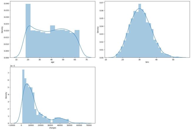
在这里，这段代码创建了一个具有预定图形大小（3行和2列）的子图网格。然后，在迭代了许多数值列（包括“age”、“bmi”和“charges”）之后，它为每一列生成一个分布图（直方图），显示DataFrame（缩写为“df”）的特定列中的值是如何分布的。然后显示子图，从而直观地了解这些数值方面的数据分布。'plt.tight_layout（）'函数用于改进子图的布局，以便更好地呈现。

数据预处理

数据预处理涉及为分析和建模准备原始数据，是数据分析和机器学习管道中的一个重要阶段。它在提高数据的准确性和可靠性方面发挥着至关重要的作用，最终提高了机器学习模型的有效性。让我们看看如何执行它：

对数转换和分布图

# Apply the natural logarithm transformation to the 'charges' column
df['charges'] = np.log1p(df['charges'])

# Create a distribution plot for the transformed 'charges' column
sb.distplot(df['charges'])

# Display the distribution plot
plt.show()

此代码中使用“np.log1p”函数对DataFrame（“df”）的“charges”列应用自然对数转换。由于这种处理，数据分布中的偏态减少了。对数转换后的值分布通过使用“sb.distplot”绘制的变化“charges”列的分布图（直方图）直观显示。然后显示分布图，该分布图提供关于改变的数据分布的细节。年龄和bmi数据是正态分布的，但费用是左偏的。我们可以对这个数据集进行对数变换，将其转换为正态分布的值。

分类列的独热编码

# Mapping Categorical to Numerical Values
 
# Map 'sex' column values ('male' to 0, 'female' to 1)
df['sex'] = df['sex'].map({'male': 0, 'female': 1})
 
# Map 'smoker' column values ('no' to 0, 'yes' to 1)
df['smoker'] = df['smoker'].map({'no': 0, 'yes': 1})
 
# Display the DataFrame's first few rows to show the transformations
df.head()

输出

    age  sex     bmi  children  smoker   charges  northeast  northwest  \
0   19  NaN  27.900         0     NaN  9.734236          0          0   
1   18  NaN  33.770         1     NaN  7.453882          0          0   
2   28  NaN  33.000         3     NaN  8.400763          0          0   
3   33  NaN  22.705         0     NaN  9.998137          0          1   
4   32  NaN  28.880         0     NaN  8.260455          0          1   
   southeast  southwest  
0          0          1  
1          1          0  
2          1          0  
3          0          0  
4          0          0  

这段代码为“sex”和“smoker”列执行分类到数字的映射，使数据适合需要数字输入的机器学习算法。它还显示DataFrame的初始行以说明更改。

# Perform one-hot encoding on the 'region' column
temp = pd.get_dummies(df['region']).astype('int')

# Concatenate the one-hot encoded columns with the original DataFrame
df = pd.concat([df, temp], axis=1)

这段代码对“region”列应用one-hot编码，将分类区域值转换为二元列，每个列表示一个不同的区域。通过将结果独热编码列与原始DataFrame连接，数据集将使用每个区域的二元特征进行扩展。

# Remove 'Id' and 'region' columns from the DataFrame
df.drop(['Id', 'region'], inplace=True, axis=1)
 
# Display the updated DataFrame
print(df.head())

输出

   age  sex     bmi  children  smoker   charges  northeast  northwest  \
0   19    1  27.900         0       1  9.734236          0          0   
1   18    0  33.770         1       0  7.453882          0          0   
2   28    0  33.000         3       0  8.400763          0          0   
3   33    0  22.705         0       0  9.998137          0          1   
4   32    0  28.880         0       0  8.260455          0          1   
   southeast  southwest  
0          0          1  
1          1          0  
2          1          0  
3          0          0  
4          0          0  

现在唯一剩下的列（分类）是区域列，让我们对它进行独热编码，因为该列中的类别数量超过2，并且名义上编码它将意味着我们在不知道现实的情况下给予偏好。

划分数据

# Define the features
features = df.drop('charges', axis=1)
 
# Define the target variable as 'charges'
target = df['charges']
 
# Split the data into training and validation sets
X_train, X_val, Y_train, Y_val = train_test_split(features, target,
                                                  random_state=2023,
                                                  test_size=0.25)
 
# Display the shapes of the training and validation sets
X_train.shape, X_val.shape

输出

((1003, 11), (335, 11))

为了在训练过程中评估模型的性能，让我们以75：25的比例分割数据集，然后用它来创建lgb数据集，然后训练模型。

特征缩放

# Standardize Features
 
# Use StandardScaler to scale the training and validation data
scaler = StandardScaler()
#Fit the StandardScaler to the training data
scaler.fit(X_train)
# transform both the training and validation data
X_train = scaler.transform(X_train)
X_val = scaler.transform(X_val)

此代码将StandardScaler拟合到训练数据以计算平均值和标准差，然后使用这些计算值转换训练和验证数据，以确保两个数据集之间的一致缩放。

# Create a LightGBM dataset for training with features X_train and labels Y_train
train_data = lgb.Dataset(X_train, label=Y_train)

# Create a LightGBM dataset for testing with features X_val and labels Y_val,
# and specify the reference dataset as train_data for consistent evaluation
test_data = lgb.Dataset(X_val, label=Y_val, reference=train_data)

现在，通过使用训练和验证数据，让我们使用lgb.Dataset创建训练和验证数据。在这里，它通过使用提供的功能和标签创建数据集对象，为lightGBM的训练和测试准备数据。

使用LightGBM的回归模型

现在剩下的最后一件事是定义一些参数，我们必须为模型的训练过程传递这些参数，以及将用于相同过程的参数。

# Define a dictionary of parameters for configuring the LightGBM regression model.
params = {
    'objective': 'regression',
    'metric': 'rmse',
    'boosting_type': 'gbdt',
    'num_leaves': 31,
    'learning_rate': 0.05,
    'feature_fraction': 0.9,
}

让我们快速查看一下传递给模型的参数。

• objective -这定义了你要训练你的模型的任务类型，例如回归已经在这里传递了回归任务，我们也可以传递分类和多类分类，用于二进制和多类分类。
• metric -模型将使用的改进指标。此外，随着训练过程的继续，我们将能够获得模型在验证数据（如果通过）上的性能。
• boosting_type -这是lightgbm模型用来训练模型参数的方法，例如GBDT（Gradient Boosting Decision Trees）是默认方法，rf（random forest based）是dart（Dropouts meet Multiple Additive Regression Trees）。
• num_leaves -默认值为31，用于定义树中叶节点的最大数量。
• learning_rate -我们知道学习率是一个非常常见的超参数，用于控制学习过程。
• feature_fraction -这是最初用于训练决策树的特征的分数。如果我们将其设置为0.9，则意味着90%的功能将仅被使用。这有助于我们处理过拟合问题。

让我们在训练数据上训练模型100个epoch，我们也将传递验证数据，以便在训练过程继续的同时可视化模型在看不见的数据上的性能。这有助于我们检查训练进度。

# Set the number of rounds and train the model with early stopping
num_round = 100
bst = lgb.train(params, train_data, num_round, valid_sets=[
                test_data], early_stopping_rounds=10)

输出

[70]    valid_0's rmse: 0.387332
[71]    valid_0's rmse: 0.387193
[72]    valid_0's rmse: 0.387407
[73]    valid_0's rmse: 0.387696
[74]    valid_0's rmse: 0.388172
[75]    valid_0's rmse: 0.388142
[76]    valid_0's rmse: 0.388688
Early stopping, best iteration is:
[66]    valid_0's rmse: 0.386691

此代码片段使用提供的参数（params）和训练数据（train_data）训练LightGBM模型，并设置boosting轮数（num_round）。使用提前停止，其中模型跟踪它在测试数据验证数据集上的表现，如果在10轮之后没有看到改进，则终止训练。这确保了模型在达到最佳性能时完成训练，并防止过拟合。在这里，我们可以观察到验证数据的均方根误差值为0.386691，这对于回归度量来说是一个非常好的分数。

模型预测与评价

# Import necessary libraries for calculating mean squared error and using the LightGBM regressor.
from sklearn.metrics import mean_squared_error as mse
from lightgbm import LGBMRegressor
 
# Create an instance of the LightGBM Regressor with the RMSE metric.
model = LGBMRegressor(metric='rmse')
 
# Train the model using the training data.
model.fit(X_train, Y_train)
 
# Make predictions on the training and validation data.
y_train = model.predict(X_train)
y_val = model.predict(X_val)

在这里，它利用lightGBM库进行回归建模。该模型在提供的训练数据上进行训练，并在训练和验证数据集上进行预测。

# Calculate and print the Root Mean Squared Error (RMSE) for training and validation predictions.
print("Training RMSE: ", np.sqrt(mse(Y_train, y_train)))
print("Validation RMSE: ", np.sqrt(mse(Y_val, y_val)))

输出

Training RMSE:  0.2331835443343122
Validation RMSE:  0.40587871797893876

在这里，该代码计算并显示了RMSE，这是一种预测准确性的度量，用于训练和验证数据集。它评估了lightGBM回归模型对数据的表现，较低的RMSE值表示更好的模型拟合。

总结

总之，利用LightGBM进行回归任务提供了一种强大而有效的预测建模方法。从数据准备和特征工程开始，该过程继续训练lightGBM回归模型，配置有特定的超参数和评估指标。该模型能够有效地从训练数据中学习，进行预测，并通过特征重要性得分提供可解释性。RMSE等评估指标有助于衡量预测的准确性。LightGBm的速度，可扩展性和强大的预测性能使其成为一个令人信服的选择，特别是处理大型数据集和在各种现实世界的应用程序中实现高质量的回归结果。