PSNR、SSIM等图像质量评估指标详解

简介：个人学习分享，如有错误，欢迎批评指正。

一、PSNR（Peak Signal-to-Noise Ratio）峰值信噪比

1. 定义

PSNR 是一种用于衡量两幅图像之间差异的客观指标。它主要用于评估图像压缩、传输或重建算法的效果。PSNR 值越高，表示两幅图像越相似，质量损失越小。

PSNR 基于信号与噪声的概念，其理论基础来自信息论中的信噪比（SNR，Signal-to-Noise Ratio）。PSNR 将图像质量的评估转化为信号（原始图像）与噪声（失真部分）的比例。

1.1 信噪比（SNR）

信噪比定义为信号功率与噪声功率的比值，通常以分贝为单位表示：

$$\text{SNR}=10\cdot {\log }_{10}\left(\frac{\text{信号功率}}{\text{噪声功率}}\right)$$
在 PSNR 中，信号功率对应于图像的最大可能像素值平方，噪声功率对应于均方误差（MSE）。

1.2 对数转换

通过对信噪比进行对数转换，PSNR 能够将大的动态范围压缩到较小的尺度，更符合人类对变化的感知。

2. 数学原理

PSNR 基于均方误差（MSE，Mean Squared Error），通过对误差进行对数转换，得到一个以分贝（dB）为单位的指标。

2.1 均方误差（MSE）

均方误差是两幅图像像素值差异的平均值，其计算公式为：

$$\text{MSE}=\frac{1}{MN}\sum _{i=1}^M\sum _{j=1}^N{\left[I_1(i,j)-I_2(i,j)\right]}^2$$

其中：

• $I_1$ 和 $I_2$ 是两幅图像，
• $M$ 和 $N$ 分别是图像的高度和宽度，
• $i$ 和 $j$ 是像素的位置索引。

2.2 PSNR 公式

有了 MSE 后，PSNR 可以通过以下公式计算：

$$\text{PSNR}=10\cdot {\log }_{10}\left(\frac{{\text{MAX}}^2}{\text{MSE}}\right)$$

其中：

• MAX 是图像中可能的最大像素值。例如，对于8位图像，MAX=255。

2.3 物理意义

PSNR 反映了信号（原图像）与噪声（失真部分）之间的比例。较高的 PSNR 值表示较少的噪声，图像质量较高。

3. 优缺点

优点

• 简单易计算：PSNR 的计算过程简单，计算效率高，适合大规模图像处理任务。
• 广泛应用：作为经典指标，许多研究和应用中都采用 PSNR 进行评估，便于结果比较。
• 明确的物理意义：PSNR 以分贝为单位，易于理解和解释。

缺点

• 感知不一致：PSNR 基于像素级误差，未能充分反映人类视觉系统对图像质量的感知。
• 忽略结构信息：PSNR 无法捕捉图像的结构、纹理等高级特征，可能导致对视觉效果的误判。
• 对噪声敏感：在某些情况下，PSNR 对特定类型的失真不敏感，无法有效区分不同失真类型。

4. 详细计算示例

假设我们有两幅 $2\times 2$ 灰度图像：

$$I_1=\left[\begin{array}{cc}52& 55\\ 61& 59\end{array}\right],I_2=\left[\begin{array}{cc}50& 54\\ 60& 58\end{array}\right]$$

4.1 计算 MSE

$$\text{MSE}=\frac{1}{2\times 2}\left((52-50{)}^2+(55-54{)}^2+(61-60{)}^2+(59-58{)}^2\right)=1.75$$

4.2 计算 PSNR

假设像素值范围为 $[0,255]$，则 $\text{MAX}=255$。

$$\text{PSNR}=10\cdot {\log }_{10}\left(\frac{255^2}{1.75}\right)\approx 10\cdot 4.568\approx 45.68\text{dB}$$

5. 示例代码

以下是使用 Python 和 OpenCV 计算 PSNR 的示例代码：

import cv2
import numpy as np

def calculate_psnr(image1_path, image2_path):
    # 读取图像
    img1 = cv2.imread(image1_path)
    img2 = cv2.imread(image2_path)

    # 检查图像尺寸是否相同
    if img1.shape != img2.shape:
        raise ValueError("输入的两幅图像必须具有相同的尺寸和通道数")

    # 计算均方误差（MSE）
    mse = np.mean((img1 - img2) ** 2)
    if mse == 0:
        return float('inf')  # 图像完全相同

    # 计算PSNR
    PIXEL_MAX = 255.0
    psnr = 10 * np.log10((PIXEL_MAX ** 2) / mse)
    return psnr

# 示例
psnr_value = calculate_psnr('image1.jpg', 'image2.jpg')
print(f"两张图像的PSNR值为: {psnr_value:.2f} dB")

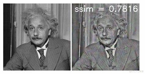
二、SSIM（Structural Similarity Index）结构相似性指数

1. 定义

SSIM 基于人类视觉系统（HVS）的感知模型，是一种用于衡量两幅图像在亮度、对比度和结构上相似度的指标。与 PSNR 不同，SSIM 更加贴近人类视觉系统的感知，能够更准确地反映图像质量。

2. 数学原理

SSIM 的核心思想是将图像看作是由亮度、对比度和结构组成的集合，通过比较这三个方面的相似性来评估整体相似度。

2.1 亮度比较

亮度是指图像的平均亮度水平，HVS 对亮度的变化具有高度敏感性。SSIM 通过比较两幅图像的平均亮度来评估相似性：

$$l(x,y)=\frac{2{\mu }_x{\mu }_y+C_1}{{\mu }_x^2+{\mu }_y^2+C_1}$$

2.2 对比度比较

对比度反映了图像中亮度变化的程度，HVS 对对比度变化同样敏感。SSIM 通过比较两幅图像的对比度来评估相似性：

$$c(x,y)=\frac{2{\sigma }_x{\sigma }_y+C_2}{{\sigma }_x^2+{\sigma }_y^2+C_2}$$

2.3 结构比较

结构反映了图像中物体的几何结构和纹理特征，HVS 对结构的感知具有高度敏感性。SSIM 通过比较两幅图像的结构相似性来评估相似性：

$$s(x,y)=\frac{{\sigma }_{xy}+C_3}{{\sigma }_x{\sigma }_y+C_3}$$

通常，$C_3$ 被设置为 $C_3=\frac{C_2}{2}$，因此 SSIM 可以简化为：

$$\text{SSIM}(x,y)={\left[l(x,y)\right]}^{\alpha }\cdot {\left[c(x,y)\right]}^{\beta }\cdot {\left[s(x,y)\right]}^{\gamma }$$

通常，$\alpha =\beta =\gamma =1$，因此：

$$\text{SSIM}(x,y)=l(x,y)\cdot c(x,y)\cdot s(x,y)$$

2.4 综合公式

将上述三个部分结合，得到 SSIM 的完整公式：

$$\text{SSIM}(x,y)=\frac{(2{\mu }_x{\mu }_y+C_1)(2{\sigma }_{xy}+C_2)}{({\mu }_x^2+{\mu }_y^2+C_1)({\sigma }_x^2+{\sigma }_y^2+C_2)}$$

其中：

• ${\mu }_x$ 和 ${\mu }_y$ 分别是图像 $x$ 和 $y$ 在局部窗口内的平均值，表示图像的亮度水平。
• ${\sigma }_x^2$ 和 ${\sigma }_y^2$ 分别是图像 $x$ 和 $y$ 在局部窗口内的方差，表示图像的对比度。
• ${\sigma }_{xy}$ 是图像 $x$ 和 $y$ 在局部窗口内的协方差，表示图像的结构相似性。
• $C_1=(K_{1}L{)}^2$，$C_2=(K_{2}L{)}^2$，通常 $K_1=0.01$，$K_2=0.03$，$L$ 是像素值的动态范围（如 8 位图像 $L=255$）。

3. 优缺点

优点

1. 符合人类视觉感知：SSIM 考虑了亮度、对比度和结构，能够更准确地反映人类对图像质量的感知。
2. 结构敏感：对图像中的结构信息变化敏感，能够有效捕捉到图像细节的变化。
3. 局部对比：通过滑动窗口的方式，SSIM 能够在局部范围内评估图像相似度，更适合评估局部失真。

缺点

1. 计算复杂度较高：相比于 PSNR，SSIM 的计算更为复杂，计算时间更长，尤其是在大规模图像处理任务中。
2. 窗口大小选择：窗口大小的选择可能影响评估结果，不同应用场景下可能需要调整。
3. 对旋转、缩放敏感：SSIM 对图像的旋转、缩放等几何变换不具备不变性，可能导致相似图像被评估为不同。

4. 详细计算示例

继续使用之前的 2x2 灰度图像示例：

$$I_1=\left[\begin{array}{cc}52& 55\\ 61& 59\end{array}\right],I_2=\left[\begin{array}{cc}50& 54\\ 60& 58\end{array}\right]$$

4.1 计算局部统计量

由于图像尺寸较小，假设使用整个图像作为一个窗口。

$${\mu }_x=\frac{52+55+61+59}{4}=\frac{227}{4}=56.75$$

$${\mu }_y=\frac{50+54+60+58}{4}=\frac{222}{4}=55.5$$

$${\sigma }_x^2=\frac{(52-56.75{)}^2+(55-56.75{)}^2+(61-56.75{)}^2+(59-56.75{)}^2}{4}=12.1875$$

$${\sigma }_y^2=\frac{(50-55.5{)}^2+(54-55.5{)}^2+(60-55.5{)}^2+(58-55.5{)}^2}{4}=14.75$$

$${\sigma }_{xy}=\frac{(52-56.75)(50-55.5)+(55-56.75)(54-55.5)+(61-56.75)(60-55.5)+(59-56.75)(58-55.5)}{4}=13.375$$

4.2 计算 SSIM

假设 $K_1=0.01$，$K_2=0.03$，$L=255$，则：

$$C_1=(0.01\times 255{)}^2=6.5025$$

$$C_2=(0.03\times 255{)}^2=58.5225$$

代入 SSIM 公式：

$$\text{SSIM}=\frac{(2\times 56.75\times 55.5+6.5025)(2\times 13.375+58.5225)}{(56.75^2+55.5^2+6.5025)(12.1875+14.75+58.5225)}\approx 0.9962$$

5. 示例代码

以下是使用 Python 计算 SSIM 的示例代码：

import cv2
import numpy as np
from scipy.ndimage import gaussian_filter

def load_image_grayscale(image_path):
    img = cv2.imread(image_path, cv2.IMREAD_GRAYSCALE)
    if img is None:
        raise ValueError(f"无法读取图像: {image_path}")
    img = img.astype(np.float64) / 255.0
    return img

def compute_statistics(img1, img2, window_size=11, sigma=1.5):
    mu1 = gaussian_filter(img1, sigma=sigma)
    mu2 = gaussian_filter(img2, sigma=sigma)
    
    sigma1_sq = gaussian_filter(img1 ** 2, sigma=sigma) - mu1 ** 2
    sigma2_sq = gaussian_filter(img2 ** 2, sigma=sigma) - mu2 ** 2
    
    sigma12 = gaussian_filter(img1 * img2, sigma=sigma) - mu1 * mu2
    
    return mu1, mu2, sigma1_sq, sigma2_sq, sigma12

def calculate_ssim(img1, img2, window_size=11, sigma=1.5, K1=0.01, K2=0.03, L=1.0):
    mu1, mu2, sigma1_sq, sigma2_sq, sigma12 = compute_statistics(img1, img2, window_size, sigma)
    
    C1 = (K1 * L) ** 2
    C2 = (K2 * L) ** 2
    
    luminance = (2 * mu1 * mu2 + C1) / (mu1 ** 2 + mu2 ** 2 + C1)
    contrast = (2 * np.sqrt(sigma1_sq) * np.sqrt(sigma2_sq) + C2) / (sigma1_sq + sigma2_sq + C2)
    structure = (sigma12 + C2 / 2) / (np.sqrt(sigma1_sq) * np.sqrt(sigma2_sq) + C2 / 2)
    
    ssim_map = luminance * contrast * structure
    return np.mean(ssim_map)

def ssim_index(image1_path, image2_path, window_size=11, sigma=1.5, K1=0.01, K2=0.03):
    img1 = load_image_grayscale(image1_path)
    img2 = load_image_grayscale(image2_path)
    
    if img1.shape != img2.shape:
        raise ValueError("输入的两幅图像必须具有相同的尺寸")
    
    ssim = calculate_ssim(img1, img2, window_size, sigma, K1, K2, L=1.0)
    return ssim

# 示例使用
if __name__ == "__main__":
    image1_path = 'original.jpg'
    image2_path = 'distorted.jpg'
    
    try:
        ssim_value = ssim_index(image1_path, image2_path)
        print(f"两张图像的SSIM值为: {ssim_value:.4f}")
    except Exception as e:
        print(f"计算SSIM时发生错误: {e}")

6. SSIM 的改进与变种

6.1 MS-SSIM（Multi-Scale SSIM）

多尺度 SSIM 通过在不同尺度下计算 SSIM，并综合各尺度的结果，提高了评估的准确性和鲁棒性。MS-SSIM 能更好地捕捉图像的全局和局部结构信息。

MS-SSIM 的计算步骤

• 多尺度分解：对图像进行多尺度分解，通常使用高斯金字塔或拉普拉斯金字塔。
• 逐尺度计算 SSIM：在每个尺度下计算 SSIM。
• 加权综合：将各尺度下的 SSIM 值加权综合，得到最终的 MS-SSIM 指标。

MS-SSIM 的优势

• 捕捉多尺度信息：能够同时考虑图像的局部和全局结构信息。
• 提高鲁棒性：对不同尺度下的图像失真具有更强的鲁棒性。

6.2 CW-SSIM（Complex Wavelet SSIM）

复数小波 SSIM 利用复数小波变换提取图像的相位信息，提高了对图像结构的捕捉能力。

CW-SSIM 的计算步骤

小波变换：对图像进行复数小波变换，提取幅度和相位信息。
相位相似性计算：通过比较相位信息，评估图像的结构相似性。
综合相似性：结合幅度和相位信息，得到 CW-SSIM 指标。

• List item

CW-SSIM 的优势

增强结构感知：通过相位信息，提高对图像结构的敏感性。
抗噪性强：对噪声和失真的鲁棒性更强。

6.3 FSIM（Feature Similarity Index）

特征相似性指数通过提取图像的低级特征（如相位一致性和梯度幅度），评估图像的相似性。

FSIM 的计算步骤

• 特征提取：提取图像的相位一致性（PC）和梯度幅度（GM）特征。
• 特征相似性计算：比较两幅图像在特征空间中的相似性。
• 综合特征相似性：通过加权融合各特征相似性，得到最终的 FSIM 指标。

FSIM 的优势

• 高精度：能够更准确地反映图像的结构和细节信息。

• 对人类视觉系统更符合：通过特征提取，更贴近 HVS 的感知机制。

6.4 VIF（Visual Information Fidelity）

视觉信息保真度通过信息论的视角，衡量图像中的可视信息量。

VIF 的计算步骤

• 图像分解：对图像进行分解，提取多尺度特征。
• 信息量计算：计算两幅图像在不同尺度下的互信息量。
• 综合信息量：通过加权融合各尺度下的互信息量，得到 VIF 指标。

VIF 的优势

• 信息理论基础：基于信息论，具有坚实的理论基础。

• 高准确性：能够准确反映图像的可视信息保留情况。

三、MSE（Mean Squared Error，均方误差）

1. 定义

均方误差(Mean Squared Error，MSE)是一种常用的图像质量评估指标，用于衡量两幅图像在像素级别上的差异。MSE通过计算两幅图像对应像素差值的平方，并取其平均值，来量化图像之间的误差。

2. 数学原理

设有两幅图像 $I_1$ 和 $I_2$，每幅图像的尺寸为 $M\times N$，即图像有 $M$ 行和 $N$ 列像素。MSE 定义为两幅图像对应像素差异的平方和的平均值，公式如下：

$$\text{MSE}=\frac{1}{MN}\sum _{i=1}^M\sum _{j=1}^N{\left[I_1(i,j)-I_2(i,j)\right]}^2$$

其中：

• $I_1(i,j)$ 和 $I_2(i,j)$ 分别表示图像 $I_1$ 和图像 $I_2$ 在位置 $(i,j)$ 处的像素值。
• $M$ 和 $N$ 分别是图像的高度和宽度。

2. MSE的优缺点

优点

• 简单易计算：MSE的计算过程直观，公式简单，易于实现。计算效率高，适合大规模图像处理任务。
• 广泛应用：作为基础误差度量，MSE在许多图像处理和计算机视觉任务中得到广泛应用，如图像压缩、图像重建和去噪。
• 数学性质良好：MSE具有良好的数学性质，如可微性，适合作为优化目标函数。

缺点

• 不符合人类视觉感知：MSE基于像素级误差度量，无法反映人类视觉系统对图像质量的感知。对于某些视觉上显著的失真，MSE可能无法准确反映其严重程度。
• 忽略结构和纹理信息：MSE仅考虑像素值差异，未能捕捉图像的结构、纹理和语义信息。对于结构性失真（如边缘模糊），MSE无法有效区分。
• 对噪声敏感：MSE对高频噪声非常敏感，即使噪声对视觉影响较小，MSE也可能显著增加。
• 单位依赖性：MSE的值依赖于像素值的范围，不同动态范围的图像MSE值不可直接比较。

3. MSE的Python实现

import cv2
import numpy as np

def calculate_mse(image1_path, image2_path):
    """
    计算两幅图像的均方误差（MSE）。
    
    参数：
    - image1_path: 第一幅图像的文件路径。
    - image2_path: 第二幅图像的文件路径。
    
    返回：
    - mse: 两幅图像的MSE值。
    """
    # 读取图像
    img1 = cv2.imread(image1_path)
    img2 = cv2.imread(image2_path)
    
    if img1 is None:
        raise ValueError(f"无法读取图像: {image1_path}")
    if img2 is None:
        raise ValueError(f"无法读取图像: {image2_path}")
    
    # 检查图像尺寸是否相同
    if img1.shape != img2.shape:
        raise ValueError("输入的两幅图像必须具有相同的尺寸和通道数")
    
    # 将图像转换为浮点型
    img1 = img1.astype(np.float64)
    img2 = img2.astype(np.float64)
    
    # 计算MSE
    mse = np.mean((img1 - img2) ** 2)
    return mse

if __name__ == "__main__":
    # 示例图像路径
    image1_path = 'original.jpg'
    image2_path = 'distorted.jpg'
    
    try:
        mse_value = calculate_mse(image1_path, image2_path)
        print(f"两张图像的MSE值为: {mse_value:.2f}")
    except Exception as e:
        print(f"计算MSE时发生错误: {e}")

四、MAE（Mean Absolute Error，平均绝对误差）

1.定义

平均绝对误差（Mean Absolute Error，MAE）是一种常用的图像质量评估指标，用于衡量两幅图像在像素级别上的差异。MAE通过计算两幅图像对应像素差值的绝对值，并取其平均值，来量化图像之间的误差。

2.数学原理

设有两幅图像 $I_1$ 和 $I_2$，每幅图像的尺寸为 $M\times N$，即图像有 $M$ 行和 $N$ 列像素。MAE 定义为两幅图像对应像素差异的绝对值和的平均值，公式如下：

$$\text{MAE}=\frac{1}{MN}\sum _{i=1}^M\sum _{j=1}^N\left|I_1(i,j)-I_2(i,j)\right|$$

其中：

• $I_1(i,j)$ 和 $I_2(i,j)$ 分别表示图像 $I_1$ 和图像 $I_2$ 在位置 $(i,j)$ 处的像素值。
• $M$ 和 $N$ 分别是图像的高度和宽度。

3. MAE的优缺点

优点

• 简单易计算：MAE的计算过程直观，公式简单，易于实现。计算效率高，适合大规模图像处理任务。
• 稳健性：相较于MSE，MAE对异常值（如噪声）的敏感性较低，具有更好的稳健性。
• 解释性强：MAE的值具有明确的物理意义，表示两幅图像在像素级别上的平均绝对差异。

缺点

• 不符合人类视觉感知：MAE基于像素级误差，无法反映人类视觉系统对图像质量的感知。对于某些视觉上显著的失真，MAE可能无法准确反映其严重程度。
• 忽略结构和纹理信息：MAE仅考虑像素值差异，未能捕捉图像的结构、纹理和语义信息。对于结构性失真（如边缘模糊），MAE无法有效区分。
• 单位依赖性：MAE的值依赖于像素值的范围，不同动态范围的图像MAE值不可直接比较。
• 线性特性：MAE对误差的线性度量，无法体现出误差的累积效应。

4. MAE的Python实现

import cv2
import numpy as np

def calculate_mae(image1_path, image2_path):
    """
    计算两幅图像的平均绝对误差（MAE）。
    
    参数：
    - image1_path: 第一幅图像的文件路径。
    - image2_path: 第二幅图像的文件路径。
    
    返回：
    - mae: 两幅图像的MAE值。
    """
    # 读取图像
    img1 = cv2.imread(image1_path)
    img2 = cv2.imread(image2_path)
    
    if img1 is None:
        raise ValueError(f"无法读取图像: {image1_path}")
    if img2 is None:
        raise ValueError(f"无法读取图像: {image2_path}")
    
    # 检查图像尺寸是否相同
    if img1.shape != img2.shape:
        raise ValueError("输入的两幅图像必须具有相同的尺寸和通道数")
    
    # 将图像转换为浮点型
    img1 = img1.astype(np.float64)
    img2 = img2.astype(np.float64)
    
    # 计算MAE
    mae = np.mean(np.abs(img1 - img2))
    return mae

if __name__ == "__main__":
    # 示例图像路径
    image1_path = 'original.jpg'
    image2_path = 'distorted.jpg'
    
    try:
        mae_value = calculate_mae(image1_path, image2_path)
        print(f"两张图像的MAE值为: {mae_value:.2f}")
    except Exception as e:
        print(f"计算MAE时发生错误: {e}")

五、UQI（Universal Quality Index，通用质量指数）

1. 定义

通用质量指数（Universal Quality Index，UQI）是由Zhou Wang等人在2002年提出的一种用于评估图像质量的指标。UQI旨在综合考虑图像的亮度、对比度和结构信息，从而更全面地反映两幅图像之间的相似度。与传统的像素级误差度量（如MSE和MAE）不同，UQI更加贴近人类视觉系统的感知。

2.数学原理

UQI通过综合衡量两幅图像在亮度、对比度和结构上的相似性，来评估图像质量。其核心思想是将这些不同的相似性度量结合起来，以提供一个统一的质量评分。

2.1 定义

设有两幅图像 $I_1$ 和 $I_2$，每幅图像的尺寸为 $M\times N$，即图像有 $M$ 行和 $N$ 列像素。UQI 定义为：

$$\text{UQI}(I_1,I_2)=\frac{4{\sigma }_{xy}{\mu }_x{\mu }_y}{({\sigma }_x^2+{\sigma }_y^2)({\mu }_x^2+{\mu }_y^2)}$$

其中：

• ${\mu }_x,{\mu }_y$ 是图像 $I_1$ 和 $I_2$ 的平均值。
• ${\sigma }_x^2,{\sigma }_y^2$ 是图像 $I_1$ 和 $I_2$ 的方差。
• ${\sigma }_{xy}$ 是图像 $I_1$ 和 $I_2$ 的协方差。

2.2 数学推导

UQI 基于以下三个关键组成部分：

1. 亮度相似性 (Luminance Similarity)：

$$l(I_1,I_2)=\frac{2{\mu }_x{\mu }_y}{{\mu }_x^2+{\mu }_y^2}$$

2. 对比度相似性 (Contrast Similarity)：

$$c(I_1,I_2)=\frac{2{\sigma }_x{\sigma }_y}{{\sigma }_x^2+{\sigma }_y^2}$$

3. 结构相似性 (Structure Similarity)：

$$s(I_1,I_2)=\frac{{\sigma }_{xy}}{{\sigma }_x{\sigma }_y}$$

UQI 将上述三个相似度量结合起来：

$$\text{UQI}(I_1,I_2)=l(I_1,I_2)\cdot c(I_1,I_2)\cdot s(I_1,I_2)=\frac{4{\sigma }_{xy}{\mu }_x{\mu }_y}{({\sigma }_x^2+{\sigma }_y^2)({\mu }_x^2+{\mu }_y^2)}$$

通过这种方式，UQI 能够同时考虑图像的亮度、对比度和结构信息，从而提供一个全面的质量评估。

3.UQI的优缺点

优点

• 综合性强：UQI同时考虑了图像的亮度、对比度和结构信息，提供了一个全面的质量评估。
• 符合视觉感知：由于考虑了结构信息，UQI更贴近人类视觉系统的感知，能够更准确地反映图像质量。
• 数学性质良好：UQI具有良好的数学性质，如对称性，易于理解和计算。
• 易于实现：相对于一些复杂的指标，UQI的计算相对简单，可以在不依赖复杂库的情况下实现。

缺点

• 对噪声敏感：UQI在存在噪声的情况下可能会受到较大影响，尤其是高频噪声。

• 忽略高阶统计特性：虽然UQI综合了亮度、对比度和结构，但它并未考虑更高阶的统计特性，如纹理和语义信息。

• 单位依赖性：UQI的值依赖于图像的像素值范围，不同动态范围的图像UQI值不可直接比较。

• 对几何变换敏感：UQI对图像的旋转、缩放等几何变换敏感，即使图像内容相同，几何变换后的图像UQI值也会较低。

4.UQI的Python实现

import cv2
import numpy as np

def calculate_uqi(image1_path, image2_path):
    """
    计算两幅图像的通用质量指数（UQI）。
    
    参数：
    - image1_path: 第一幅图像的文件路径。
    - image2_path: 第二幅图像的文件路径。
    
    返回：
    - uqi: 两幅图像的UQI值。
    """
    # 读取图像
    img1 = cv2.imread(image1_path)
    img2 = cv2.imread(image2_path)
    
    if img1 is None:
        raise ValueError(f"无法读取图像: {image1_path}")
    if img2 is None:
        raise ValueError(f"无法读取图像: {image2_path}")
    
    # 检查图像尺寸是否相同
    if img1.shape != img2.shape:
        raise ValueError("输入的两幅图像必须具有相同的尺寸和通道数")
    
    # 将图像转换为浮点型，并归一化到[0,1]范围
    img1 = img1.astype(np.float64) / 255.0
    img2 = img2.astype(np.float64) / 255.0
    
    # 计算平均值
    mu_x = np.mean(img1, axis=(0,1))
    mu_y = np.mean(img2, axis=(0,1))
    
    # 计算方差
    sigma_x_sq = np.var(img1, axis=(0,1))
    sigma_y_sq = np.var(img2, axis=(0,1))
    
    # 计算协方差
    sigma_xy = np.mean((img1 - mu_x) * (img2 - mu_y), axis=(0,1))
    
    # 计算UQI每个通道
    numerator = 4 * sigma_xy * mu_x * mu_y
    denominator = (sigma_x_sq + sigma_y_sq) * (mu_x**2 + mu_y**2)
    
    # 防止除以零
    denominator = np.where(denominator == 0, 1e-10, denominator)
    
    uqi_channels = numerator / denominator
    
    # 取平均UQI
    uqi = np.mean(uqi_channels)
    
    return uqi

if __name__ == "__main__":
    # 示例图像路径
    image1_path = 'original.jpg'
    image2_path = 'distorted.jpg'
    
    try:
        uqi_value = calculate_uqi(image1_path, image2_path)
        print(f"两张图像的UQI值为: {uqi_value:.4f}")
    except Exception as e:
        print(f"计算UQI时发生错误: {e}")

六、FSIM（Feature Similarity Index，特征相似性指数）

1.定义

特征相似性指数（FSIM）由Zhang等人在2011年提出，是一种基于低级特征（如相位一致性和梯度幅度）的图像质量评估指标。FSIM旨在更好地模拟人类视觉系统（HVS）的感知，通过比较图像的关键特征来衡量相似度。

2.数学原理

FSIM基于以下两个关键特征：

1. 相位一致性（Phase Consistency）：

   • 描述图像局部区域的结构信息。
   • 通过傅里叶变换提取图像的相位信息，以捕捉边缘和纹理。

2. 梯度幅度（Gradient Magnitude）：

   • 反映图像的对比度和边缘强度。

   • 通过计算图像的梯度来衡量局部对比度。

FSIM通过结合这两种特征的相似性，提供一个全面的质量评估。

FSIM 的计算公式如下：

$$\text{FSIM}(I_1,I_2)=\frac{{\sum }_x\varphi (x)\cdot {\text{SIM}}_G(x)}{{\sum }_x\varphi (x)}$$

其中：

• $\varphi (x)$ 是相位一致性函数。
• ${\text{SIM}}_G(x)$ 是梯度幅度的相似性函数。

计算步骤

1. 相位一致性计算：

   • 对两幅图像进行傅里叶变换，提取相位信息。
   • 计算相位一致性函数 $\varphi (x)$。

2. 梯度幅度计算：

   • 计算两幅图像的梯度幅度 $G_1$ 和 $G_2$。
   • 计算梯度幅度相似性函数 ${\text{SIM}}_G(x)$。

3. 结合相似性：

   • 将相位一致性与梯度幅度相似性结合，得到 FSIM 值。

3. FSIM的优缺点

优点

• 高精度：考虑了相位和梯度特征，能够更准确地反映图像的结构和细节。
• 符合人类视觉感知：模拟了HVS对图像结构和对比度的敏感性。
• 鲁棒性强：对各种失真类型（如模糊、噪声、压缩失真）具有良好的评估能力。

缺点

• 计算复杂：涉及傅里叶变换和梯度计算，计算量较大。
• 参数选择敏感：需要合理设置参数以适应不同应用场景。
• 对几何变换敏感：如旋转、缩放等变换会影响FSIM值。

4.FSIM的Python实现

import cv2
import numpy as np

def calculate_fsim(image1_path, image2_path):
    """
    计算两幅图像的特征相似性指数（FSIM）。
    
    参数：
    - image1_path: 第一幅图像的文件路径。
    - image2_path: 第二幅图像的文件路径。
    
    返回：
    - fsim: 两幅图像的FSIM值。
    """
    # 读取图像并转换为灰度
    img1 = cv2.imread(image1_path, cv2.IMREAD_GRAYSCALE).astype(np.float64)
    img2 = cv2.imread(image2_path, cv2.IMREAD_GRAYSCALE).astype(np.float64)
    
    if img1.shape != img2.shape:
        raise ValueError("输入的两幅图像必须具有相同的尺寸")
    
    # 计算相位一致性
    def phase_consistency(img1, img2):
        F1 = np.fft.fft2(img1)
        F2 = np.fft.fft2(img2)
        phase1 = np.angle(F1)
        phase2 = np.angle(F2)
        phi = (2 * (phase1 * phase2 + 1)) / (phase1**2 + phase2**2 + 1)
        return phi
    
    phi = phase_consistency(img1, img2)
    
    # 计算梯度幅度
    def gradient_magnitude(img):
        grad_x = cv2.Sobel(img, cv2.CV_64F, 1, 0, ksize=3)
        grad_y = cv2.Sobel(img, cv2.CV_64F, 0, 1, ksize=3)
        magnitude = np.sqrt(grad_x**2 + grad_y**2)
        return magnitude
    
    G1 = gradient_magnitude(img1)
    G2 = gradient_magnitude(img2)
    
    # 计算梯度相似性
    eps = 1e-10
    sim_G = (2 * G1 * G2 + eps) / (G1**2 + G2**2 + eps)
    
    # 计算FSIM
    fsim_map = phi * sim_G
    fsim = np.mean(fsim_map)
    
    return fsim

if __name__ == "__main__":
    image1_path = 'original.jpg'
    image2_path = 'distorted.jpg'
    
    try:
        fsim_value = calculate_fsim(image1_path, image2_path)
        print(f"两张图像的FSIM值为: {fsim_value:.4f}")
    except Exception as e:
        print(f"计算FSIM时发生错误: {e}")

七、GMSD（Gradient Magnitude Similarity Deviation，梯度幅度相似性偏差）

1.定义

梯度幅度相似性偏差（GMSD）由Zhang等人在2015年提出，是一种基于梯度幅度的图像质量评估指标。GMSD旨在通过比较两幅图像的梯度幅度图，量化它们之间的视觉差异，提供快速且有效的质量评估。

2.数学原理

GMSD基于梯度幅度相似性，其核心思想是通过比较图像的梯度信息来评估图像质量。梯度幅度反映了图像中的边缘和细节信息，是衡量图像结构的重要特征。

核心步骤

1. 梯度幅度计算：使用Sobel算子或其他梯度算子计算原始图像和失真图像的梯度幅度。
2. 梯度幅度相似性：计算两幅图像对应梯度幅度的相似性，通常使用归一化的梯度幅度相似性函数。
3. 偏差计算：计算所有像素点的梯度幅度相似性偏差的平均值，得到GMSD值。

2.1 基本公式

GMSD 的计算公式如下：

$$\text{GMSD}=\sqrt{\frac{\frac{1}{MN}{\sum }_{i=1}^M{\sum }_{j=1}^N{\left(S(x,y)-\hat{S}(x,y)\right)}^2}{{\mu }_S}}$$

其中：

• $S(x,y)$ 和 $\hat{S}(x,y)$ 分别是原始图像和失真图像在像素 $(x,y)$ 处的梯度幅度。
• $M$ 和 $N$ 是图像的高度和宽度。
• ${\mu }_S$ 是原始图像梯度幅度的平均值。

3.2 示例计算

假设有两幅 $3\times 3$ 的灰度图像，计算其 GMSD：

1. 计算梯度幅度（使用简化的 Sobel 算子）：

原始图像 $I$：

I = [ 52 55 60 61 59 58 62 60 57 ] I = \begin{bmatrix} 52 & 55 & 60 \\ 61 & 59 & 58 \\ 62 & 60 & 57 \end{bmatrix} I= ​526162​555960​605857​ ​

失真图像 $\hat{I}$：

I ^ = [ 50 54 59 60 58 57 61 59 56 ] \hat{I} = \begin{bmatrix} 50 & 54 & 59 \\ 60 & 58 & 57 \\ 61 & 59 & 56 \end{bmatrix} I^= ​506061​545859​595756​ ​

1. 计算梯度幅度 $S$ 和 $\hat{S}$（简化示例，实际使用 Sobel 算子）：

S = [ 5 5 5 5 5 5 5 5 5 ] , S ^ = [ 5 5 5 5 5 5 5 5 5 ] S = \begin{bmatrix} 5 & 5 & 5 \\ 5 & 5 & 5 \\ 5 & 5 & 5 \end{bmatrix}, \quad \hat{S} = \begin{bmatrix} 5 & 5 & 5 \\ 5 & 5 & 5 \\ 5 & 5 & 5 \end{bmatrix} S= ​555​555​555​ ​,S^= ​555​555​555​ ​

---

2. 计算相似性偏差：

( S − S ^ ) 2 = [ 0 0 0 0 0 0 0 0 0 ] (S - \hat{S})^2 = \begin{bmatrix} 0 & 0 & 0 \\ 0 & 0 & 0 \\ 0 & 0 & 0 \end{bmatrix} (S−S^)2= ​000​000​000​ ​

---

3. 计算 GMSD：

$$\text{GMSD}=\sqrt{\frac{\frac{0}{9}}{5}}=0$$

3. GMSD的优缺点

优点

• 高效性：计算简单，适合大规模图像处理任务。
• 符合视觉感知：基于梯度信息，能够有效捕捉图像的边缘和细节，符合人类对图像质量的感知。
• 鲁棒性：对多种失真类型（如模糊、噪声、压缩失真）具有良好的评估能力。

缺点

• 对噪声敏感：高频噪声会影响梯度幅度的计算，可能导致GMSD值不准确。
• 忽略颜色信息：主要基于灰度图像的梯度幅度，未充分利用彩色图像的颜色信息。
• 局部信息缺失：对图像局部区域的质量变化不够敏感，可能忽略细微的局部失真。

4.GMSD的Python实现

import cv2
import numpy as np
import os

def calculate_gmsd(image1_path, image2_path):
    """
    计算两幅图像的梯度幅度相似性偏差（GMSD）。
    
    参数：
    - image1_path: 第一幅图像的文件路径。
    - image2_path: 第二幅图像的文件路径。
    
    返回：
    - gmsd: 两幅图像的GMSD值。
    """
    # 读取图像并转换为灰度
    img1 = cv2.imread(image1_path, cv2.IMREAD_GRAYSCALE).astype(np.float64)
    img2 = cv2.imread(image2_path, cv2.IMREAD_GRAYSCALE).astype(np.float64)
    
    if img1.shape != img2.shape:
        raise ValueError("输入的两幅图像必须具有相同的尺寸")
    
    # 计算梯度幅度（使用Sobel算子）
    def gradient_magnitude(img):
        grad_x = cv2.Sobel(img, cv2.CV_64F, 1, 0, ksize=3)
        grad_y = cv2.Sobel(img, cv2.CV_64F, 0, 1, ksize=3)
        magnitude = np.sqrt(grad_x**2 + grad_y**2)
        return magnitude
    
    G1 = gradient_magnitude(img1)
    G2 = gradient_magnitude(img2)
    
    # 计算相似性
    eps = 1e-10
    sim_map = (2 * G1 * G2 + eps) / (G1**2 + G2**2 + eps)
    
    # 计算GMSD
    gmsd = np.sqrt(np.mean((sim_map - 1) ** 2)) / np.mean(G1)
    
    return gmsd

def calculate_gmsd_batch(original_dir, distorted_dir):
    """
    批量计算两组图像的梯度幅度相似性偏差（GMSD）。
    
    参数：
    - original_dir: 原始图像文件夹路径。
    - distorted_dir: 失真图像文件夹路径。
    
    返回：
    - gmsd_results: 字典，包含每对图像的GMSD值。
    """
    gmsd_results = {}
    original_images = sorted(os.listdir(original_dir))
    distorted_images = sorted(os.listdir(distorted_dir))
    
    if len(original_images) != len(distorted_images):
        raise ValueError("原始图像和失真图像的数量必须相同")
    
    for orig, dist in zip(original_images, distorted_images):
        orig_path = os.path.join(original_dir, orig)
        dist_path = os.path.join(distorted_dir, dist)
        
        try:
            gmsd = calculate_gmsd(orig_path, dist_path)
            gmsd_results[(orig, dist)] = gmsd
        except Exception as e:
            print(f"处理图像对 ({orig}, {dist}) 时发生错误: {e}")
    
    return gmsd_results

if __name__ == "__main__":
    original_dir = 'original_images'
    distorted_dir = 'distorted_images'
    
    try:
        gmsd_results = calculate_gmsd_batch(original_dir, distorted_dir)
        for (orig, dist), gmsd in gmsd_results.items():
            print(f"图像对 ({orig}, {dist}) 的GMSD值为: {gmsd:.4f}")
    except Exception as e:
        print(f"批量计算GMSD时发生错误: {e}")

八、LPIPS（Learned Perceptual Image Patch Similarity，学习感知图像块相似度）

1.定义

学习感知图像块相似度（LPIPS）由Zhang等人在2018年提出，是一种基于深度学习的图像质量评估指标。LPIPS旨在通过深度神经网络提取图像的高级特征，并比较这些特征的相似度，以更好地模拟人类视觉系统（HVS）的感知。

2.数学原理

LPIPS基于深度神经网络（通常是预训练的卷积神经网络，如AlexNet、VGG等）提取图像的多层特征。通过比较两幅图像在这些特征层的相似性，LPIPS能够捕捉到更高级的语义和结构信息，超越传统的像素级误差度量。

核心步骤

1. 特征提取：使用预训练的深度网络提取两幅图像的多层特征表示。
2. 特征比较：对应层的特征图进行逐元素比较，计算相似性度量（通常使用L2距离）。
3. 加权融合：学习到的权重用于加权不同层的相似性度量，综合得到最终的LPIPS评分。

基本公式

LPIPS 的计算公式可以表示为：

$$\text{LPIPS}(I_1,I_2)=\sum _l{w}_l\cdot \Vert {\varphi }_l(I_1)-{\varphi }_l(I_2){\Vert }_2$$

其中：

• ${\varphi }_l(I)$ 是第 $l$ 层的特征提取函数。
• $w_l$ 是学习到的权重。
• $\Vert \cdot {\Vert }_2$ 表示 L2 范数。

3. LPIPS的优缺点

优点

• 高感知相关性：能更好地模拟人类视觉系统，捕捉高级语义和结构信息。
• 鲁棒性强：对多种失真类型（如模糊、噪声、压缩失真）具有良好的评估能力。
• 灵活性高：可通过选择不同的预训练网络和层数，适应不同的应用需求。

缺点

• 计算复杂：需要深度神经网络的前向传播，计算资源需求高。
• 依赖预训练模型：需要使用预训练的深度网络，且结果依赖于所选模型的特性。
• 训练需求：学习权重需要大量的带标签数据，训练过程复杂。

4.LPIPS的Python实现

import lpips
import torch
import cv2
import numpy as np
import os

def calculate_lpips_batch(original_dir, distorted_dir, model='vgg'):
    """
    批量计算两组图像的学习感知图像块相似度（LPIPS）。
    
    参数：
    - original_dir: 原始图像文件夹路径。
    - distorted_dir: 失真图像文件夹路径。
    - model: 使用的预训练模型（'alex', 'vgg', 等）。
    
    返回：
    - lpips_results: 字典，包含每对图像的LPIPS值。
    """
    lpips_results = {}
    original_images = sorted(os.listdir(original_dir))
    distorted_images = sorted(os.listdir(distorted_dir))
    
    if len(original_images) != len(distorted_images):
        raise ValueError("原始图像和失真图像的数量必须相同")
    
    # 加载LPIPS模型
    loss_fn = lpips.LPIPS(net=model)
    
    for orig, dist in zip(original_images, distorted_images):
        orig_path = os.path.join(original_dir, orig)
        dist_path = os.path.join(distorted_dir, dist)
        
        try:
            # 预处理
            def preprocess(img_path):
                img = cv2.imread(img_path)
                if img is None:
                    raise ValueError(f"无法读取图像: {img_path}")
                img = cv2.cvtColor(img, cv2.COLOR_BGR2RGB)
                img = cv2.resize(img, (256, 256))  # 调整大小
                img = img.astype(np.float32) / 255.0
                img = torch.from_numpy(img).permute(2, 0, 1).unsqueeze(0)
                return img

            img1 = preprocess(orig_path)
            img2 = preprocess(dist_path)
            
            # 计算LPIPS
            with torch.no_grad():
                lpips_val = loss_fn(img1, img2).item()
            
            lpips_results[(orig, dist)] = lpips_val
        except Exception as e:
            print(f"处理图像对 ({orig}, {dist}) 时发生错误: {e}")
    
    return lpips_results

if __name__ == "__main__":
    original_dir = 'original_images'
    distorted_dir = 'distorted_images'
    
    try:
        lpips_results = calculate_lpips_batch(original_dir, distorted_dir, model='vgg')
        for (orig, dist), lpips_val in lpips_results.items():
            print(f"图像对 ({orig}, {dist}) 的LPIPS值为: {lpips_val:.4f}")
    except Exception as e:
        print(f"批量计算LPIPS时发生错误: {e}")

九、DISTS（Deep Image Structure and Texture Similarity，深度图像结构与纹理相似性）

1.定义

深度图像结构与纹理相似性（DISTS）由Zhang等人在2020年提出，是一种基于深度学习的图像质量评估指标。DISTS结合了图像的结构和纹理信息，通过深度神经网络提取特征，旨在更准确地模拟人类视觉系统（HVS）的感知。

2.数学原理

DISTS基于深度神经网络（如VGG）提取图像的多层特征，通过比较这些特征的结构和纹理相似性，量化两幅图像的质量差异。

核心组成部分

• 结构相似性（Structure Similarity）：利用深层特征捕捉图像的整体结构信息。
• 纹理相似性（Texture Similarity）：通过浅层特征捕捉图像的纹理细节。
• 加权融合：结合结构和纹理相似性，综合评估图像质量。

2.1 基本公式

DISTS 的计算公式可以表示为：

$$\text{DISTS}(I_1,I_2)=\alpha \cdot \text{Structure}(I_1,I_2)+(1-\alpha )\cdot \text{Texture}(I_1,I_2)$$

其中：

• $\text{Structure}(I_1,I_2)$：结构相似度量。
• $\text{Texture}(I_1,I_2)$：纹理相似度量。
• $\alpha$：权重系数，用于平衡结构与纹理的重要性。

2.2 计算步骤

1. 特征提取：使用预训练的深度网络（如VGG）提取原始图像和失真图像的多层特征。
2. 相似性度量：计算对应层特征的结构和纹理相似性，通常使用L2距离或其他相似性指标。
3. 加权融合：根据预设的权重系数α，结合结构与纹理相似性，得到最终的DISTS评分。

3. DISTS的优缺点

优点

• 高感知相关性：结合结构和纹理信息，更贴近人类视觉感知。
• 鲁棒性强：对多种失真类型（如模糊、噪声、压缩失真）具有良好的评估能力。
• 综合性强：同时考虑图像的全局结构和局部纹理，提供全面的质量评估。

缺点

• 计算复杂：依赖深度神经网络的前向传播，计算资源需求高。
• 依赖预训练模型：结果依赖于所选深度网络的特性和训练数据。
• 参数调整：需要合理设置权重系数 α，以适应不同应用场景。

4.DISTS的Python实现

import torch
import torchvision.transforms as transforms
from PIL import Image
from dists import DISTS
import os

def calculate_dists_batch(original_dir, distorted_dir, model='vgg'):
    """
    批量计算两组图像的深度图像结构与纹理相似性（DISTS）。
    
    参数：
    - original_dir: 原始图像文件夹路径。
    - distorted_dir: 失真图像文件夹路径。
    - model: 使用的预训练模型（'vgg', 'alex', 等）。
    
    返回：
    - dists_results: 字典，包含每对图像的DISTS值。
    """
    dists_results = {}
    original_images = sorted(os.listdir(original_dir))
    distorted_images = sorted(os.listdir(distorted_dir))
    
    if len(original_images) != len(distorted_images):
        raise ValueError("原始图像和失真图像的数量必须相同")
    
    # 图像预处理
    transform = transforms.Compose([
        transforms.Resize((256, 256)),
        transforms.ToTensor(),
    ])
    
    # 加载DISTS模型
    dists_model = DISTS(model=model).eval()
    
    for orig, dist in zip(original_images, distorted_images):
        orig_path = os.path.join(original_dir, orig)
        dist_path = os.path.join(distorted_dir, dist)
        
        try:
            img1 = Image.open(orig_path).convert('RGB')
            img2 = Image.open(dist_path).convert('RGB')
            
            img1 = transform(img1).unsqueeze(0)
            img2 = transform(img2).unsqueeze(0)
            
            with torch.no_grad():
                dists_val = dists_model(img1, img2).item()
            
            dists_results[(orig, dist)] = dists_val
        except Exception as e:
            print(f"处理图像对 ({orig}, {dist}) 时发生错误: {e}")
    
    return dists_results

if __name__ == "__main__":
    original_dir = 'original_images'
    distorted_dir = 'distorted_images'
    
    try:
        dists_results = calculate_dists_batch(original_dir, distorted_dir, model='vgg')
        for (orig, dist), dists_val in dists_results.items():
            print(f"图像对 ({orig}, {dist}) 的DISTS值为: {dists_val:.4f}")
    except Exception as e:
        print(f"批量计算DISTS时发生错误: {e}")

十、IFC（Information Fidelity Criterion，信息保真度准则）

1.定义

信息保真度准则（IFC）由Sheikh和Cohen在2005年提出，是一种基于信息理论的图像质量评估指标。IFC旨在衡量失真图像中保留的与原始图像相关的有用信息量，提供对图像质量的客观评估。

2.数学原理

IFC基于信息理论，具体采用信源编码理论和信息保真度的概念。核心思想是通过比较原始图像和失真图像之间的信息传递，评估失真图像中保留的原始信息量。

核心概念

• 信息保真度：衡量失真图像中保留的与原始图像相关的信息量。
• 信源模型：原始图像被视为信源，通过信道传输后产生失真图像。
• 熵和互信息：使用熵（信息量）和互信息（两变量间共享的信息量）来量化信息保真度。

2.1 基本公式

IFC 的计算基于互信息的概念，其基本公式为：

$$\text{IFC}(I,K)=\frac{I(I;K)}{I(I;K)+I(N;K)}$$

其中：

• $I$ 是原始图像。
• $K$ 是失真图像。
• $N$ 是噪声图像（噪声与原始图像无关）。
• $I(A;B)$ 表示 $A$ 和 $B$ 之间的互信息。

2.2 计算步骤

1. 信源建模：将原始图像和失真图像建模为随机变量。
2. 概率分布估计：估计原始图像和失真图像的联合概率分布。
3. 互信息计算：计算原始图像与失真图像之间的互信息 $I(I;K)$，计算噪声图像与失真图像之间的互信息$I(N;K)$。
4. IFC计算：将互信息代入IFC公式，得到最终的IFC值。

3.IFC的优缺点

优点

• 理论基础坚实：基于信息理论，具有良好的数学基础和理论支持。
• 信息量衡量：能够量化失真图像中保留的有用信息量，提供直观的质量评估。
• 鲁棒性强：对多种失真类型（如压缩、噪声、模糊）具有良好的评估能力。

缺点

• 计算复杂：需要估计高维的概率分布，计算量大，效率较低。
• 依赖模型假设：信源和信道的建模依赖于假设，实际应用中可能不完全符合。
• 缺乏普适性：在某些失真类型或图像内容下，IFC的评估可能不够准确。

4.IFC的Python实现

import cv2
import numpy as np
from sklearn.metrics import mutual_info_score

def calculate_ifc(original_path, distorted_path, bins=256):
    """
    计算两幅图像的信息保真度准则（IFC）。
    
    参数：
    - original_path: 原始图像的文件路径。
    - distorted_path: 失真图像的文件路径。
    - bins: 直方图的箱数。
    
    返回：
    - ifc: 两幅图像的IFC值。
    """
    # 读取图像并转换为灰度
    img1 = cv2.imread(original_path, cv2.IMREAD_GRAYSCALE)
    img2 = cv2.imread(distorted_path, cv2.IMREAD_GRAYSCALE)
    
    if img1 is None or img2 is None:
        raise ValueError("无法读取图像文件。")
    if img1.shape != img2.shape:
        raise ValueError("输入的两幅图像必须具有相同的尺寸。")
    
    # 计算互信息
    def mutual_information(img1, img2, bins):
        hist_2d, _, _ = np.histogram2d(img1.ravel(), img2.ravel(), bins=bins)
        mi = mutual_info_score(None, None, contingency=hist_2d)
        return mi
    
    mi_ik = mutual_information(img1, img2, bins)
    # 假设噪声图像与失真图像无关，互信息为0
    mi_nk = 0
    
    # 计算IFC
    ifc = mi_ik / (mi_ik + mi_nk + 1e-10)  # 加小值防止除零
    
    return ifc

if __name__ == "__main__":
    original_path = 'original.jpg'
    distorted_path = 'distorted.jpg'
    
    try:
        ifc_value = calculate_ifc(original_path, distorted_path)
        print(f"两张图像的IFC值为: {ifc_value:.4f}")
    except Exception as e:
        print(f"计算IFC时发生错误: {e}")

十一、总结和对比

1.选择建议：

• 任务需求：

  • 像素级精度：如果任务需要评估像素级误差，如图像压缩和重建，可以使用PSNR和MSE。
  • 结构和感知质量：如果任务需要更符合人类视觉感知的评估，如图像超分辨率和去噪，建议使用SSIM、LPIPS或FSIM。
  • 高级特征：对于需要考虑高级特征和语义信息的任务，可以使用基于深度学习的指标，如LPIPS和DISTS。

• 计算资源：

  • 高效评估：对于需要快速评估的场景，如实时图像处理，可以选择PSNR、MSE或GMSD。

  • 高精度评估：对于离线评估或对质量要求较高的任务，可以选择SSIM、LPIPS或FSIM。

• 应用场景：

  • 医学影像：需要高精度和结构信息的保留，可以选择SSIM、VIF或IFC。
  • 监控与安全：需要快速评估，可以选择PSNR、MSE或GMSD。

2.对比总结

指标	优点	缺点	适用场景
MSE	计算简单，数学性质良好	不符合人类视觉感知，忽略结构和纹理信息，对异常值敏感	基础图像处理任务，如压缩、重建
MAE	简单易计算，稳健性较好	不符合人类视觉感知，忽略结构和纹理信息	基础图像处理任务，如压缩、重建、快速评估
PSNR	基于 MSE，易于理解，广泛应用	同 MSE，仍然不符合人类视觉感知，无法反映结构信息	图像压缩、重建的初步评估
SSIM	考虑亮度、对比度和结构，符合人类视觉感知	计算复杂，对几何变换敏感	高精度图像质量评估、图像增强、超分辨率等
UQI	综合考虑亮度、对比度和结构信息，符合人类视觉感知	计算复杂，对噪声敏感，忽略高阶特征	高级图像质量评估、图像压缩、重建、去噪
VIF	基于信息理论，准确反映图像信息保留情况	计算复杂，依赖标准库支持	信息保真要求较高的图像评估
FSIM	高精度，考虑结构和细节信息，符合人类视觉系统	计算复杂，需提取特定特征	需要高精度和细节保留的图像质量评估
GMSD	简单有效，计算效率高，对结构变化敏感	仅基于梯度信息，可能忽略其他视觉特征	快速图像质量评估、结构变化检测
LPIPS	更符合人类感知，能够捕捉高级语义信息	需要预训练深度模型，计算资源需求高	生成模型评估、超分辨率、图像增强
DISTS	综合考虑结构和纹理信息，更全面的质量评估	需要预训练深度模型，计算资源需求高	高级图像质量评估、结构和纹理保留
IFC	基于信息理论，准确反映有用信息保留情况	计算复杂，缺乏标准库支持	医学影像、高精度信息保留的图像评估

在实际应用中，结合使用多种指标能够提供更全面的评估。例如，使用PSNR和SSIM可以同时衡量像素级误差和结构相似性，再结合LPIPS评估感知质量，以获得更准确的图像质量评估。

---

结~~~