matlab实现gabor filter (5)

gabor filter源代码：

 

%%%%%%%VERSION 2
%%ANOTHER DESCRIBTION OF GABOR FILTER

%The Gabor filter is basically a Gaussian (with variances sx and sy along x and y-axes respectively)
%modulated by a complex sinusoid (with centre frequencies U and V along x and y-axes respectively) 
%described by the following equation
%%
%                            -1     x' ^     y'  ^             
%%% G(x,y,theta,f) =  exp ([----{(----) 2+(----) 2}])*cos(2*pi*f*x');
%                             2    sx'       sy'
%%% x' = x*cos(theta)+y*sin(theta);
%%% y' = y*cos(theta)-x*sin(theta);

%% Describtion :

%% I : Input image
%% Sx & Sy : Variances along x and y-axes respectively
%% f : The frequency of the sinusoidal function
%% theta : The orientation of Gabor filter

%% G : The output filter as described above
%% gabout : The output filtered image



%%  Author : Ahmad poursaberi  e-mail : [email protected]
%%          Faulty of Engineering, Electrical&Computer Department,Tehran
%%          University,Iran,June 2004

function [G,gabout] = gaborfilter1(I,Sx,Sy,f,theta)

if isa(I,'double')~=1 
    I = double(I);
end

for x = -fix(Sx):fix(Sx)
    for y = -fix(Sy):fix(Sy)
        xPrime = x * cos(theta) + y * sin(theta);
        yPrime = y * cos(theta) - x * sin(theta);
        G(fix(Sx)+x+1,fix(Sy)+y+1) = exp(-.5*((xPrime/Sx)^2+(yPrime/Sy)^2))*cos(2*pi*f*xPrime);
    end
end

Imgabout = conv2(I,double(imag(G)),'same');
Regabout = conv2(I,double(real(G)),'same');

gabout = sqrt(Imgabout.*Imgabout + Regabout.*Regabout);

 

调用代码：

 

close all;
clear all;
clc;

% 读入图像
image=imread('C:\Users\watkins\Pictures\cartoon.jpg');
grayImage=rgb2gray(image);
grayImage=im2double(grayImage);
% 显示读入图像
imshow(grayImage);

sx=32;
sy=32;
theta=[0 pi/4 2*pi/4 3*pi/4 4*pi/4 5*pi/4 6*pi/4 7*pi/4];
gamma=1;
psi=0;
sigma=6; % 也可以为12
lambda=[5 6 7 8 9];

V=[4 5 6 7 8];
U=[0 pi/4 2*pi/4 3*pi/4 4*pi/4 5*pi/4 6*pi/4 7*pi];
%U=[1 2 3 4 5 6 7 8];

% Creating 40 Gabor Filters
G = cell(5,8);
for i = 1:5
    for j = 1:8
        G{i,j}=zeros(65,65);
    end
end
for i = 1:5
    for j = 1:8
        f=1/lambda(i);
        %[T,gabout] = gaborfilter(grayImage,sx,sy,U(j),V(i));
        %G{i,j} = T;
        G{i,j} = gaborfilter1(grayImage,sx,sy,f,theta(j));
    end
end

% Showing Gabor Filters
figure;
for s = 1:5
    for j = 1:8        
        subplot(5,8,(s-1)*8+j);        
        %imshow(real(G{s,j})/2-0.5,[]);
        imshow(real(G{s,j}),[]);
    end
end

 

显示的滤波器组图片：

 

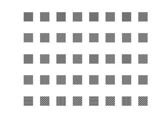
可以明显看到波长和方向的变化