机器学习--分类算法（一）决策树

转：http://www.cnblogs.com/zhangchaoyang/articles/2196631.html

一、算法

Key points:

• 决策树是一个分类算法，分类结果是离散值（对应输出结果是连续值的回归算法）；
• 有监督的分类算法;
• 是一种贪婪算法，生成的每一步都是局部最优值
• 容易over fitting
• noise影响不大
• 空间划分，通过递归的方法把特征空间划分成不重叠的矩形

如何处理过拟合的问题：

• Pre-pruning：

        - 设定一个阈值，该阈值可以是决策树高度，节点实例个数，信息增益值等，该节点成为叶节点

        - 该叶节点持有其数据集中样本最多的类或者其概率分布 

• Post-pruning：

        -    首先构造完整的决策树，允许决策树过度拟合训练数据

       - 对置信度不够的节点的子树用叶节点或树枝来替代

       - 该叶节点持有其子树的数据集中样本最多的类或者其概率分布

什么时候需要剪枝：

1. 数据噪音，因此有的分类不准
2. 训练数据量少，或者不具有代表性
3. 过拟合

ID3, C4.5, C5.0, CART

ID3 1986年 Quilan

选择具有最高信息增益的属性作为测试属性

01 ID3(DataSet, featureList):
02   - 创建根节点R
03   - 如果当前DataSet中的数据都属于同一类，则标记R的类别为该类
04   - 如果当前featureList集合为空，则标记R的类别为当前DataSet中样本最多的类别
05   - 递归情况：
06     # 从featureList中选择属性（选择Gain(DataSet,F)最大的属性）
07     # 根据F的每一个值v,将DataSet划分为不同的子集DS，对每一个Ds:
08       - 创建节点C
09       - 如果DS为空，节点C标记为DataSet中样本最多的类别
10       - 如果DS不为空，节点C=ID3（DS,featureList-F）
11       - 将节点C添加为R的子节点

C4.5 1993年 by Quilab(对ID3的改进)

• 信息增益率（information gain ratio）
• 连续值属性

           离散化处理：将连续型的属性变量进行离散化处理，形成决策树的训练集

               - 把需要处理的样本按照连续变量的大小从小到大进行排序

               - 假设该属性对应的不同的属性值一共有N个，那么总共有N-1个可能的候选分割阈值点，每个候选的分割阈值点的值为上述排序后的属性值中两两前后元素的中点

               - 用信息增益率选择最佳划分

• 缺失值

        - 处理缺少属性值的一种策略是赋给它节点t所对应的训练实例中该属性的最常见值

        - 复杂一点的办法是为每个可能值赋一个概率

        - 最简单的办法是丢弃这些样本

• 后剪枝（基于错误剪枝EBP-Error Based Pruning）

    

C5.0 1998年

加入了Boosting算法框架

CART (Classification and Regression Trees)

• 二元划分

        - 二叉树不易产生数据碎片，精确度往往会高于多叉树，所以在CART算法中采用二元划分  

• 不纯性度量

        - 分类目标：Gini指标、Towing、order Towing

        - 连续目标：最小平方残差、最小绝对残差

• 剪枝

        - 用独立的验证数据集对训练集生长的树进行剪枝

分类树：    

01 CART_classification(DataSet, featureList, alpha,)：
02 创建根节点R
03 如果当前DataSet中的数据的类别相同，则标记R的类别标记为该类
04 如果决策树高度大于alpha，则不再分解，标记R的类别classify(DataSet)
05 递归情况：
06 标记R的类别classify(DataSet)
07 从featureList中选择属性F（选择Gini(DataSet, F)最小的属性划分，连续属性参考C4.5的离散化过程(以Gini最小作为划分标准)）
08 根据F，将DataSet做二元划分DS_L 和 DS_R：
09 如果DS_L或DS_R为空，则不再分解
10 如果DS_L和DS_R都不为空，节点
11     C_L= CART_classification(DS_L, featureList, alpha);
12     C_R= CART_classification(DS_R featureList, alpha)
13 将节点C_L和C_R添加为R的左右子节点

回归树

01 CART_regression(DataSet, featureList, alpha, delta)：
02 创建根节点R
03 如果当前DataSet中的数据的值都相同，则标记R的值为该值
04 如果最大的phi值小于设定阈值delta，则标记R的值为DataSet应变量均值
05 如果其中一个要产生的节点的样本数量小于alpha，则不再分解，标记R的值为DataSet应变量均值
06 递归情况：
07 从featureList中选择属性F（选择phi(DataSet, F)最大的属性，连续属性（或使用多个属性的线性组合）参考C4.5的离散化过程 (以phi最大作为划分标准)）
08 根据F，将DataSet做二元划分DS_L 和 DS_R：
09 如果DS_L或DS_R为空，则标记节点R的值为DataSet应变量均值
10 如果DS_L和DS_R都不为空，节点
11     C_L= CART_regression(DS_L, featureList, alpha, delta);
12     C_R= CART_regression(DS_R featureList, alpha, delta)
13 将节点C_L和C_R添加为R的左右子节点

分类树与回归树的差别在于空间划分方法一个是线性一个是非线性

先上问题吧，我们统计了14天的气象数据(指标包括outlook，temperature，humidity，windy)，并已知这些天气是否打球(play)。如果给出新一天的气象指标数据:sunny,cool,high,TRUE，判断一下会不会去打球。

table 1

outlook	temperature	humidity	windy	play
sunny	hot	high	FALSE	no
sunny	hot	high	TRUE	no
overcast	hot	high	FALSE	yes
rainy	mild	high	FALSE	yes
rainy	cool	normal	FALSE	yes
rainy	cool	normal	TRUE	no
overcast	cool	normal	TRUE	yes
sunny	mild	high	FALSE	no
sunny	cool	normal	FALSE	yes
rainy	mild	normal	FALSE	yes
sunny	mild	normal	TRUE	yes
overcast	mild	high	TRUE	yes
overcast	hot	normal	FALSE	yes
rainy	mild	high	TRUE	no

这个问题当然可以用朴素贝叶斯法求解，分别计算在给定天气条件下打球和不打球的概率，选概率大者作为推测结果。

现在我们使用ID3归纳决策树的方法来求解该问题。

预备知识：信息熵

熵是无序性（或不确定性）的度量指标。假如事件A的全概率划分是（A1,A2,...,An），每部分发生的概率是(p1,p2,...,pn)，那信息熵定义为：

通常以2为底数，所以信息熵的单位是bit。

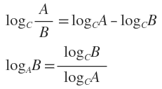
补充两个对数去处公式：

上文中，我们提到：“ID3算法的核心思想就是以信息增益度量属性选择，选择分裂后信息增益( 很快，由下文你就会知道信息增益又是怎么一回事)最大的属性进行分裂。”接下来，咱们就来看看这个信息增益是个什么概念( 当然，在了解信息增益之前，你必须先理解：信息增益的度量标准：熵)。

    上述的ID3算法的核心问题是选取在树的每个结点要测试的属性。我们希望选择的是最有利于分类实例的属性，信息增益(Information Gain)是用来 衡量给定的属性区分训练样例的能力，而ID3算法在增长树的每一步使用信息增益从候选属性中选择属性。

    为了精确地定义信息增益，我们先定义信息论中广泛使用的一个度量标准，称为熵（entropy），它刻画了任意样例集的纯度（purity）。给定包含关于某个目标概念的正反样例的样例集S，那么S相对这个布尔型分类的熵为：

    上述公式中，p+代表正样例，比如在本文开头第二个例子中p+则意味着去打羽毛球，而p-则代表反样例，不去打球(在有关熵的所有计算中我们定义0log0为0)。

    如果写代码实现熵的计算，则如下所示：

 //根据具体属性和值来计算熵
 double ComputeEntropy(vector <vector <string> > remain_state, string attribute, string value,bool ifparent){
     vector<int> count (2,0);
     unsigned int i,j;
     bool done_flag = false;//哨兵值
     for(j = 1; j < MAXLEN; j++){
         if(done_flag) break;
         if(!attribute_row[j].compare(attribute)){
             for(i = 1; i < remain_state.size(); i++){
                 if((!ifparent&&!remain_state[i][j].compare(value)) || ifparent){//ifparent记录是否算父节点
                     if(!remain_state[i][MAXLEN - 1].compare(yes)){
                         count[0]++;
                     }
                     else count[1]++;
                 }
             }
             done_flag = true;
         }
     }
     if(count[0] == 0 || count[1] == 0 ) return 0;//全部是正实例或者负实例
     //具体计算熵 根据[+count[0],-count[1]],log2为底通过换底公式换成自然数底数
     double sum = count[0] + count[1];
     double entropy = -count[0]/sum*log(count[0]/sum)/log(2.0) - count[1]/sum*log(count[1]/sum)/log(2.0);
     return entropy;
 }

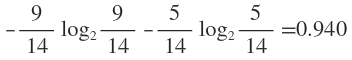
    举例来说，假设S是一个关于布尔概念的有14个样例的集合，它包括9个正例和5个反例（我们采用记号[9+，5-]来概括这样的数据样例），那么S相对于这个布尔样例的熵为：

Entropy（[9+，5-]）=-（9/14）log2（9/14）-（5/14）log2（5/14）=0.940。

     So，根据上述这个公式，我们可以得到：S的所有成员属于同一类，Entropy(S)=0； S的正反样例数量相等，Entropy(S)=1；S的正反样例数量不等，熵介于0，1之间，如下图所示：

    信息论中对熵的一种解释，熵确定了要编码集合S中任意成员的分类所需要的最少二进制位数。更一般地，如果目标属性具有c个不同的值，那么S相对于c个状态的分类的熵定义为：

     Pi为子集合中不同性(而二元分类即正样例和负样例)的样例的比例。【参考：http://blog.csdn.net/v_july_v/article/details/7577684】

ID3算法

构造树的基本想法是随着树深度的增加，节点的熵迅速地降低。熵降低的速度越快越好，这样我们有望得到一棵高度最矮的决策树。

在没有给定任何天气信息时，根据历史数据，我们只知道新的一天打球的概率是9/14，不打的概率是5/14。此时的熵为：

属性有4个：outlook，temperature，humidity，windy。我们首先要决定哪个属性作树的根节点。

对每项指标分别统计：在不同的取值下打球和不打球的次数。

table 2

outlook			temperature			humidity			windy			play
	yes	no		yes	no		yes	no		yes	no	yes	no
sunny	2	3	hot	2	2	high	3	4	FALSE	6	2	9	5
overcast	4	0	mild	4	2	normal	6	1	TRUR	3	3
rainy	3	2	cool	3	1

下面我们计算当已知变量outlook的值时，信息熵为多少。

outlook=sunny时，2/5的概率打球，3/5的概率不打球。entropy=0.971

outlook=overcast时，entropy=0

outlook=rainy时，entropy=0.971

而根据历史统计数据，outlook取值为sunny、overcast、rainy的概率分别是5/14、4/14、5/14，所以当已知变量outlook的值时，信息熵为：5/14 × 0.971 + 4/14 × 0 + 5/14 × 0.971 = 0.693

这样的话系统熵就从0.940下降到了0.693，信息增溢gain(outlook)为0.940-0.693=0.247

同样可以计算出gain(temperature)=0.029，gain(humidity)=0.152，gain(windy)=0.048。

gain(outlook)最大（即outlook在第一步使系统的信息熵下降得最快），所以决策树的根节点就取outlook。

接下来要确定N1取temperature、humidity还是windy?在已知outlook=sunny的情况，根据历史数据，我们作出类似table 2的一张表，分别计算gain(temperature)、gain(humidity)和gain(windy)，选最大者为N1。

依此类推，构造决策树。当系统的信息熵降为0时，就没有必要再往下构造决策树了，此时叶子节点都是纯的--这是理想情况。最坏的情况下，决策树的高度为属性（决策变量）的个数，叶子节点不纯（这意味着我们要以一定的概率来作出决策）。

Java实现

最终的决策树保存在了XML中，使用了Dom4J，注意如果要让Dom4J支持按XPath选择节点，还得引入包jaxen.jar。程序代码要求输入文件满足ARFF格式，并且属性都是标称变量。【这个下载很多，都不太好用，附上下载链接

dom4j-1.6.1.zip：http://vdisk.weibo.com/s/dyBeYCrADepB8  


jaxen-1.1.6-bin.ziphttp://vdisk.weibo.com/s/dyBeYCrADepBd】

实验用的数据文件：

@relation weather.symbolic
 
@attribute outlook {sunny, overcast, rainy}
@attribute temperature {hot, mild, cool}
@attribute humidity {high, normal}
@attribute windy {TRUE, FALSE}
@attribute play {yes, no}
 
@data
sunny,hot,high,FALSE,no
sunny,hot,high,TRUE,no
overcast,hot,high,FALSE,yes
rainy,mild,high,FALSE,yes
rainy,cool,normal,FALSE,yes
rainy,cool,normal,TRUE,no
overcast,cool,normal,TRUE,yes
sunny,mild,high,FALSE,no
sunny,cool,normal,FALSE,yes
rainy,mild,normal,FALSE,yes
sunny,mild,normal,TRUE,yes
overcast,mild,high,TRUE,yes
overcast,hot,normal,FALSE,yes
rainy,mild,high,TRUE,no

实验代码：

package classify;

import java.io.BufferedReader;
import java.io.File;
import java.io.FileReader;
import java.io.FileWriter;
import java.io.IOException;
import java.util.ArrayList;
import java.util.Iterator;
import java.util.LinkedList;
import java.util.List;
import java.util.regex.Matcher;
import java.util.regex.Pattern;

import org.dom4j.Document;
import org.dom4j.DocumentHelper;
import org.dom4j.Element;
import org.dom4j.io.OutputFormat;
import org.dom4j.io.XMLWriter;
 
public class ID3 {
    private ArrayList<String> attribute = new ArrayList<String>(); // 存储属性的名称
    private ArrayList<ArrayList<String>> attributevalue = new ArrayList<ArrayList<String>>(); // 存储每个属性的取值
    private ArrayList<String[]> data = new ArrayList<String[]>();; // 原始数据
    int decatt; // 决策变量在属性集中的索引
    public static final String patternString = "@attribute(.*)[{](.*?)[}]";
 
    Document xmldoc;
    Element root;
 
    public ID3() {
        xmldoc = DocumentHelper.createDocument();
        root = xmldoc.addElement("root");
        root.addElement("DecisionTree").addAttribute("value", "null");
    }
 
    public static void main(String[] args) {
        ID3 inst = new ID3();
        inst.readARFF(new File("d:\\weather.nominal.arff"));
        inst.setDec("play");
        LinkedList<Integer> ll=new LinkedList<Integer>();
        for(int i=0;i<inst.attribute.size();i++){
            if(i!=inst.decatt)
                ll.add(i);
        }
        ArrayList<Integer> al=new ArrayList<Integer>();
        for(int i=0;i<inst.data.size();i++){
            al.add(i);
        }
        inst.buildDT("DecisionTree", "null", al, ll);
        inst.writeXML("d:\\dt.xml");
        return;
    }
 
    //读取arff文件，给attribute、attributevalue、data赋值
    public void readARFF(File file) {
        try {
            FileReader fr = new FileReader(file);
            BufferedReader br = new BufferedReader(fr);
            String line;
            Pattern pattern = Pattern.compile(patternString);
            while ((line = br.readLine()) != null) {
                Matcher matcher = pattern.matcher(line);
                if (matcher.find()) {
                    attribute.add(matcher.group(1).trim());
                    String[] values = matcher.group(2).split(",");
                    ArrayList<String> al = new ArrayList<String>(values.length);
                    for (String value : values) {
                        al.add(value.trim());
                    }
                    attributevalue.add(al);
                } else if (line.startsWith("@data")) {
                    while ((line = br.readLine()) != null) {
                        if(line=="")
                            continue;
                        String[] row = line.split(",");
                        data.add(row);
                    }
                } else {
                    continue;
                }
            }
            br.close();
        } catch (IOException e1) {
            e1.printStackTrace();
        }
    }
 
    //设置决策变量
    public void setDec(int n) {
        if (n < 0 || n >= attribute.size()) {
            System.err.println("决策变量指定错误。");
            System.exit(2);
        }
        decatt = n;
    }
    public void setDec(String name) {
        int n = attribute.indexOf(name);
        setDec(n);
    }
 
    //给一个样本（数组中是各种情况的计数），计算它的熵
    public double getEntropy(int[] arr) {
        double entropy = 0.0;
        int sum = 0;
        for (int i = 0; i < arr.length; i++) {
            entropy -= arr[i] * Math.log(arr[i]+Double.MIN_VALUE)/Math.log(2);
            sum += arr[i];
        }
        entropy += sum * Math.log(sum+Double.MIN_VALUE)/Math.log(2);
        entropy /= sum;
        return entropy;
    }
 
    //给一个样本数组及样本的算术和，计算它的熵
    public double getEntropy(int[] arr, int sum) {
        double entropy = 0.0;
        for (int i = 0; i < arr.length; i++) {
            entropy -= arr[i] * Math.log(arr[i]+Double.MIN_VALUE)/Math.log(2);
        }
        entropy += sum * Math.log(sum+Double.MIN_VALUE)/Math.log(2);
        entropy /= sum;
        return entropy;
    }
 
    public boolean infoPure(ArrayList<Integer> subset) {
        String value = data.get(subset.get(0))[decatt];
        for (int i = 1; i < subset.size(); i++) {
            String next=data.get(subset.get(i))[decatt];
            //equals表示对象内容相同，==表示两个对象指向的是同一片内存
            if (!value.equals(next))
                return false;
        }
        return true;
    }
 
    // 给定原始数据的子集(subset中存储行号),当以第index个属性为节点时计算它的信息熵
    public double calNodeEntropy(ArrayList<Integer> subset, int index) {
        int sum = subset.size();
        double entropy = 0.0;
        int[][] info = new int[attributevalue.get(index).size()][];
        for (int i = 0; i < info.length; i++)
            info[i] = new int[attributevalue.get(decatt).size()];
        int[] count = new int[attributevalue.get(index).size()];
        for (int i = 0; i < sum; i++) {
            int n = subset.get(i);
            String nodevalue = data.get(n)[index];
            int nodeind = attributevalue.get(index).indexOf(nodevalue);
            count[nodeind]++;
            String decvalue = data.get(n)[decatt];
            int decind = attributevalue.get(decatt).indexOf(decvalue);
            info[nodeind][decind]++;
        }
        for (int i = 0; i < info.length; i++) {
            entropy += getEntropy(info[i]) * count[i] / sum;
        }
        return entropy;
    }
 
    // 构建决策树
    public void buildDT(String name, String value, ArrayList<Integer> subset,
            LinkedList<Integer> selatt) {
        Element ele = null;
        @SuppressWarnings("unchecked")
        List<Element> list = root.selectNodes("//"+name);
        Iterator<Element> iter=list.iterator();
        while(iter.hasNext()){
            ele=iter.next();
            if(ele.attributeValue("value").equals(value))
                break;
        }
        if (infoPure(subset)) {
            ele.setText(data.get(subset.get(0))[decatt]);
            return;
        }
        int minIndex = -1;
        double minEntropy = Double.MAX_VALUE;
        for (int i = 0; i < selatt.size(); i++) {
            if (i == decatt)
                continue;
            double entropy = calNodeEntropy(subset, selatt.get(i));
            if (entropy < minEntropy) {
                minIndex = selatt.get(i);
                minEntropy = entropy;
            }
        }
        String nodeName = attribute.get(minIndex);
        selatt.remove(new Integer(minIndex));
        ArrayList<String> attvalues = attributevalue.get(minIndex);
        for (String val : attvalues) {
            ele.addElement(nodeName).addAttribute("value", val);
            ArrayList<Integer> al = new ArrayList<Integer>();
            for (int i = 0; i < subset.size(); i++) {
                if (data.get(subset.get(i))[minIndex].equals(val)) {
                    al.add(subset.get(i));
                }
            }
            buildDT(nodeName, val, al, selatt);
        }
    }
 
    // 把xml写入文件
    public void writeXML(String filename) {
        try {
            File file = new File(filename);
            if (!file.exists())
                file.createNewFile();
            FileWriter fw = new FileWriter(file);
            OutputFormat format = OutputFormat.createPrettyPrint(); // 美化格式
            XMLWriter output = new XMLWriter(fw, format);
            output.write(xmldoc);
            output.close();
        } catch (IOException e) {
            System.out.println(e.getMessage());
        }
    }
}

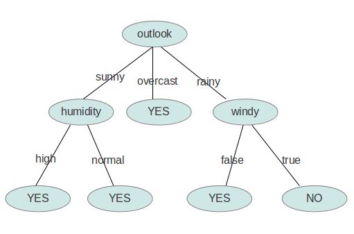
实验结果

<?xml version="1.0" encoding="UTF-8"?>

<root>
  <DecisionTree value="null">
    <outlook value="sunny">
      <humidity value="high">no</humidity>
      <humidity value="normal">yes</humidity>
    </outlook>
    <outlook value="overcast">yes</outlook>
    <outlook value="rainy">
      <windy value="TRUE">no</windy>
      <windy value="FALSE">yes</windy>
    </outlook>
  </DecisionTree>
</root>

用图形象地表示就是：【左边high对应的是NO】