scikit-learn 学习总结 （一）——sklearn实现感知机（perceptron）

学习《python machine learning》 的第三章，A Tour of Machine Learning Classifiers Using scikit-learn

本章主要讲述 特征选择 和 数据预处理，以下算法实现都是基于sklearn的接口~~~~

生命不息，学习不止~ 哈哈哈哈

【训练一个机器学习模型的五大关键步骤：】

（1）选择特征，收集训练样本

（2）选择性能指标

（3）选择分类器和优化算法

（4）评估模型性能

（5）调整算法（调参）

【training a percetron】

sklearn中自带了一些数据集，比如iris数据集，Iris数据中data存储花瓣长宽（column0,1）和花萼长宽（column2,3）.

target存储花的分类，Iris-setosa , Iris-versicolor , and Iris-virginica ，分别存储为数字 0,1,2

【收集训练样本】

from sklearn import datasets
import numpy as np

iris = datasets.load_iris()
X = iris.data[:,[2, 3]]
y = iris.target
print(np.unique(y))

【  train_test_split   分为训练集和测试集】

train_test_split 将数据集分为训练集和测试集，test_size参数决定测试集的比例。

random_state参数是随机数生成种子，在分类前将数据打乱，保证数据的可重复利用。

stratify 保证训练集和测试集中花的三大类的比例与输入比例相同。

【验证分层分类 stratification】

from sklearn.model_selection import train_test_split
#train_test_split
X_train, X_test, y_train, y_test = train_test_split(X, y, test_size = 0.3, 
                                                    random_state = 1, stratify = y )
#bincount
print("Labels counts in y: ",np.bincount(y))
print("Labels counts in y_train: ", np.bincount(y_train))
print("Labels counts in y_test: ", np.bincount(y_test))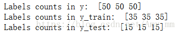

【特征标准化 Standardize the feature】

运用sklearn preprocessing模块的StandardScaler类对特征值进行标准化

StandardScaler( )函数参考自

http://scikit-learn.org/stable/modules/generated/sklearn.preprocessing.StandardScaler.html

fit ( )函数计算平均值和标准差

transform（）运用fit计算的mean和std deviation 进行数据的标准化

from sklearn.preprocessing import StandardScaler
sc = StandardScaler()
sc.fit(X_train)
X_train_std = sc.transform(X_train)
X_test_std = sc.transform(X_test)

【train perceptron model】

#train perceptron model
from sklearn.linear_model import Perceptron
ppn = Perceptron(n_iter = 40, eta0 = 0.1, random_state = 1)
ppn.fit(X_train_std, y_train)

y_pred = ppn.predict(X_test_std)
miss_classified = (y_pred != y_test).sum()
print("MissClassified: ",miss_classified)

【metrics model 选择新能指标】

accuracy_score 

from sklearn.metrics import accuracy_score
print('Accuracy : % .2f' % accuracy_score(y_pred, y_test))

或者 Perceptron.score() ——结合predict()函数和accuracy_score()函数 返回感知机的预测正确率

参数为predict的参数

print("Accuracy Score : % .2f" % ppn.score(X_test_std,y_test))

【画分离超平面】

#画超平面

from matplotlib.colors import ListedColormap
import matplotlib.pyplot as plt

def plot_decision_regions(X, y, classifier, test_idx=None, resolution=0.02):

    # setup marker generator and color map
    markers = ('s', 'x', 'o', '^', 'v')
    colors = ('red', 'blue', 'lightgreen', 'gray', 'cyan')
    cmap = ListedColormap(colors[:len(np.unique(y))])

    # plot the decision surface
    x1_min, x1_max = X[:, 0].min() - 1, X[:, 0].max() + 1
    x2_min, x2_max = X[:, 1].min() - 1, X[:, 1].max() + 1
    xx1, xx2 = np.meshgrid(np.arange(x1_min, x1_max, resolution),
                           np.arange(x2_min, x2_max, resolution))
    Z = classifier.predict(np.array([xx1.ravel(), xx2.ravel()]).T)
    Z = Z.reshape(xx1.shape)
    plt.contourf(xx1, xx2, Z, alpha=0.3, cmap=cmap)
    plt.xlim(xx1.min(), xx1.max())
    plt.ylim(xx2.min(), xx2.max())

    for idx, cl in enumerate(np.unique(y)):
        plt.scatter(x=X[y == cl, 0], 
                    y=X[y == cl, 1],
                    alpha=0.8, 
                    c=colors[idx],
                    marker=markers[idx], 
                    label=cl, 
                    edgecolor='black')

    # highlight test samples
    if test_idx:
        # plot all samples
        X_test, y_test = X[test_idx, :], y[test_idx]

        plt.scatter(X_test[:, 0],
                    X_test[:, 1],
                    c='',
                    edgecolor='black',
                    alpha=1.0,
                    linewidth=1,
                    marker='o',
                    s=100, 
                    label='test set')

#htack vstack 水平叠加和垂直叠加
X_combined_std = np.vstack((X_train_std,X_test_std))
y_combined_std = np.hstack((y_train, y_test))
plot_decision_regions(X = X_combined_std, 
                      y = y_combined_std, 
                      classifier = ppn, 
                      test_idx = range(105,150))
plt.xlabel('petal length [standardized]')
plt.ylabel('petal width [standardized]')
plt.legend(loc = 'upper left')
plt.tight_layout()
plt.show()

 

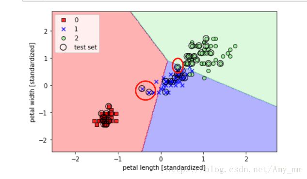
可以看到圈出的三个错误分类点（我圈出的，不是plot出来的）~~~

感知机只能对线性数据进行正确分类，对于非线性数据，可以采用逻辑回归等分类方法。见下一篇博文 ——sklearn实现逻辑回归。