Gabor滤波详解

先搬运定义

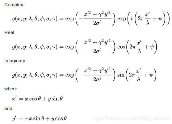
Its impulse response is defined by a sinusoidal wave (a plane wave for 2D Gabor filters) multiplied by a Gaussian function. Because of the multiplication-convolution property (Convolution theorem), the Fourier transform of a Gabor filter's impulse response is the convolution of the Fourier transform of the harmonic function (sinusoidal function) and the Fourier transform of the Gaussian function. The filter has a real and an imaginary component representing orthogonal directions. The two components may be formed into a complex number or used individually.

In this equation, {lambda } represents the wavelength of the sinusoidal factor, {theta } represents the orientation of the normal to the parallel stripes of a Gabor function, {psi } is the phase offset, {sigma } is the sigma/standard deviation of the Gaussian envelope and {gamma } is the spatial aspect ratio, and specifies the ellipticity of the support of the Gabor function.

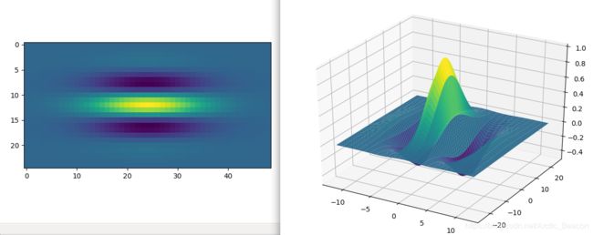
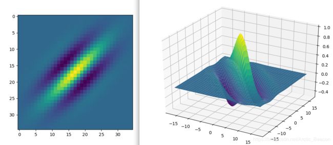
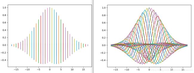
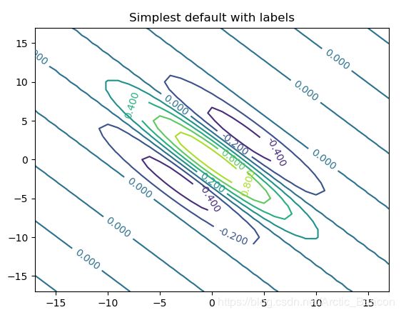
滤波器可视化

import numpy as np
import matplotlib.pyplot as plt
from matplotlib import cm
from mpl_toolkits.mplot3d import Axes3D
from matplotlib.ticker import LinearLocator, FormatStrFormatter

def gabor_fn(sigma, theta, Lambda, psi, gamma):
    sigma_x = sigma
    sigma_y = float(sigma) / gamma

    # Bounding box
    nstds = 3 # Number of standard deviation sigma
    xmax = max(abs(nstds * sigma_x * np.cos(theta)), abs(nstds * sigma_y * np.sin(theta)))
    xmax = np.ceil(max(1, xmax))
    ymax = max(abs(nstds * sigma_x * np.sin(theta)), abs(nstds * sigma_y * np.cos(theta)))
    ymax = np.ceil(max(1, ymax))
    xmin = -xmax
    ymin = -ymax
    (y, x) = np.meshgrid(np.arange(ymin, ymax + 1), np.arange(xmin, xmax + 1))

    # Rotation 
    x_theta = x * np.cos(theta) + y * np.sin(theta)
    y_theta = -x * np.sin(theta) + y * np.cos(theta)

    gb = np.exp(-.5 * (x_theta ** 2 / sigma_x ** 2 + y_theta ** 2 / sigma_y ** 2)) * np.cos(2 * np.pi / Lambda * x_theta + psi)
    return x,y,gb

x,y,gb = gabor_fn(4,0,10,0,0.5)

plt.figure()
plt.imshow(gb)

fig, ax = plt.subplots()
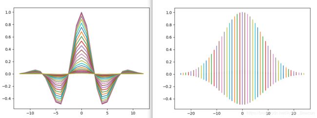
ax.plot(x, gb, '-')
plt.show()

fig, ax = plt.subplots()
ax.plot(y, gb, '-')
plt.show()

fig, ax = plt.subplots()
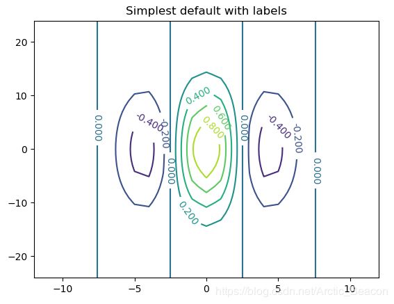
CS = ax.contour(x, y, gb)
ax.clabel(CS, inline=1, fontsize=10)
ax.set_title('Simplest default with labels')


fig = plt.figure()
ax = Axes3D(fig)
ax.plot_surface(x, y, gb, rstride=1, cstride=1, cmap=cm.viridis)

plt.show()

 

 

上述是theta = 0的滤波器，下面看看theta = pi/4

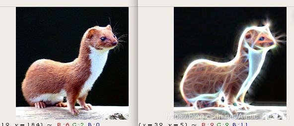
filter band滤波图像

import numpy as np
import cv2
import sys

 
def build_filters():
    filters = []
    ksize = 31
    for theta in np.arange(0, np.pi, np.pi / 16):
        kern = cv2.getGaborKernel((ksize, ksize), 4.0, theta, 10.0, 0.5, 0, ktype=cv2.CV_32F)
        kern /= 1.5*kern.sum()
        filters.append(kern)
    return filters
 
def process(img, filters):
    accum = np.zeros_like(img)
    for kern in filters:
        fimg = cv2.filter2D(img, cv2.CV_8UC3, kern)
        np.maximum(accum, fimg, accum)
    return accum
 
if __name__ == '__main__':

 
    print (__doc__)
    try:
        img_fn = sys.argv[1]
    except:
        img_fn = 'laska.png'
 
    img = cv2.imread(img_fn)
    if img is None:
        print ('Failed to load image file:', img_fn)
        sys.exit(1)
 
    filters = build_filters()
 
    res1 = process(img, filters)
    cv2.imshow('origin',img)
    cv2.imshow('result', res1)