高斯分布和卡方分布
高斯分布和卡方分布
- 高斯分布和卡方分布
- 高斯分布
- 1 单元高斯分布
- 1.1 一维随机变量
- 1.2 标准正太分布
- 1.3 numpy中使用正太分布
- 2 多元高斯分布
- 2.1 独立多元/维高斯分布
- 2.2 举例-画2维独立不相关高斯图
- 2.3 相关系数
- 2.3 举例-画2维不独立相关高斯图
高斯分布和卡方分布
高斯分布
1 单元高斯分布
1.1 一维随机变量
定义:若连续型随机变量 X X X的概率密度为
(1.1) f ( x ) = 1 2 π σ e − ( x − μ ) 2 2 σ 2 , − ∞ < x < ∞ , f(x)=\frac{1}{\sqrt{2\pi}\sigma}e^{-\frac{(x-\mu)^2}{2\sigma^2}}, -\infty<x<\infty,\tag{1.1} f(x)=2πσ1e−2σ2(x−μ)2,−∞<x<∞,(1.1)
其中 μ , σ ( σ > 0 ) \mu,\sigma(\sigma>0) μ,σ(σ>0)为常数,则称 X X X服从参数为 μ , σ \mu,\sigma μ,σ的正太/高斯分布,记为 X ∼ N ( μ , σ 2 ) X\sim N(\mu,\sigma^2) X∼N(μ,σ2).
性质:
- f ( x ) ≥ 0 f(x)\ge 0 f(x)≥0
- ∫ − ∞ ∞ f ( x ) d x = 1 \int_{-\infty}^{\infty}f(x)dx=1 ∫−∞∞f(x)dx=1
下图为均值为 μ , 均 方 根 为 σ \mu,均方根为\sigma μ,均方根为σ的高斯分布图,峰值最大值为 f ( x ) m a x = 1 2 π σ , x = μ . f(x)_{max}=\frac{1}{\sqrt{2\pi}\sigma}, x=\mu. f(x)max=2πσ1,x=μ.

特点:
- 如果固定方差 σ 2 \sigma^2 σ2, 改变参数 μ \mu μ,则正太曲线沿着 x x x轴平行移动,而图形的形状不改变。
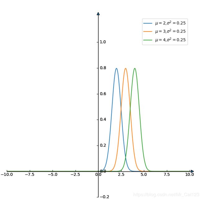
这个问题很容易想明白,因为均值 μ \mu μ是跟 ( x − μ ) (x-\mu) (x−μ)一起的,因此 ( x − ( μ + δ ) ) = ( ( x − δ ) − μ ) (x-(\mu+\delta))=((x-\delta)-\mu) (x−(μ+δ))=((x−δ)−μ), 即对 x x x做了平移处理。
import numpy as np
import matplotlib.pyplot as plt
import mpl_toolkits.axisartist as axisartist

#定义坐标轴函数
def setup_axes(fig, rect):
    ax = axisartist.Subplot(fig, rect)
    fig.add_axes(ax)

    ax.set_ylim(-.2, 1.2)
    #自定义刻度
#    ax.set_yticks([-10, 0,9])
    ax.set_xlim(-10,10)
    ax.axis[:].set_visible(False)

	#第2条线,即y轴,经过x=0的点
    ax.axis["y"] = ax.new_floating_axis(1, 0)
    ax.axis["y"].set_axisline_style("-|>", size=1.5)
#    第一条线,x轴,经过y=0的点
    ax.axis["x"] = ax.new_floating_axis(0, 0)
    ax.axis["x"].set_axisline_style("-|>", size=1.5)

    return(ax)

def gaussian(x,mu,sigma):
    f_x = np.exp(-np.power(x-mu, 2.)/(2*np.power(sigma,2.)))
    return(f_x)

#设置画布
fig = plt.figure(figsize=(8, 8)) #建议可以直接plt.figure()不定义大小
ax1 = setup_axes(fig, 111)
ax1.axis["x"].set_axis_direction("bottom")
ax1.axis['y'].set_axis_direction('right')

#在已经定义好的画布上加入高斯函数

x_values = np.linspace(-20,20,2000)
for mu,sigma in [(2,3),(3,3),(4,3)]:
   plt.plot(x_values,gaussian(x_values,mu,sigma),label=r'$\mu=$'+str(mu)+',$\sigma^2=3$')

plt.show()
- 如果固定 μ \mu μ, 改变参数 σ \sigma σ,由于峰值最大值为 f ( x ) m a x = 1 2 π σ f(x)_{max}=\frac{1}{\sqrt{2\pi}\sigma} f(x)max=2πσ1,所以 σ \sigma σ变小则图形“尖瘦”,反之“矮胖”

for mu,sigma in [(2,0.5),(2,2),(2,3)]:
    plt.plot(x_values,gaussian(x_values,mu,sigma),label=r'$\mu=2$'+',$\sigma^2=$'+str(sigma**2))
1.2 标准正太分布
特别的, 当 μ = 0 , σ = 1 \mu=0,\sigma=1 μ=0,σ=1时随机变量 X X X服从标准正太分布,记为 X ∼ N ( 0 , 1 ) X\sim N(0,1) X∼N(0,1),分布密度和分布函数为:
f ( x ) = 1 2 π e − x 2 2 , − ∞ < x < ∞ f(x)=\frac{1}{\sqrt{2\pi}}e^{-\frac{x^2}{2}}, -\infty<x<\infty f(x)=2π1e−2x2,−∞<x<∞
F ( x ) = 1 2 π ∫ − ∞ x e − t 2 2 d t , − ∞ < x < ∞ F(x)=\frac{1}{\sqrt{2\pi}}\int_{-\infty}^{x}e^{-\frac{t^2}{2}}dt,- \infty<x<\infty F(x)=2π1∫−∞xe−2t2dt,−∞<x<∞
注意分布密度函数 F ( x ) F(x) F(x)是 x x x的函数而不是 t t t的函数,因为 t t t被积分掉了,而 x x x才是变化的量。
一般的,对于 X ∼ N ( μ , σ 2 ) X\sim N(\mu,\sigma^2) X∼N(μ,σ2)的分布函数,可通过线性变换化成标准正太分布形式。
F ( x ) = ∫ − ∞ x 1 σ 2 π e − ( t − μ ) 2 2 σ 2 d t F(x)=\int_{-\infty}^{x}\frac{1}{\sigma\sqrt{2\pi}}e^{-\frac{(t-\mu)^2}{2\sigma^2}}dt F(x)=∫−∞xσ2π1e−2σ2(t−μ)2dt
令 y = t − u σ y=\frac{t-u}{\sigma} y=σt−u,可得
F ( x ) = ∫ − ∞ x − μ σ 1 2 π e − y 2 2 d y F(x)=\int_{-\infty}^{\frac{x-\mu}{\sigma}}\frac{1}{\sqrt{2\pi}}e^{-\frac{y^2}{2}}dy F(x)=∫−∞σx−μ2π1e−2y2dy
(上面利用 d y = d ( t − μ σ ) = d t σ dy=d(\frac{t-\mu}{\sigma})=d\frac{t}{\sigma} dy=d(σt−μ)=dσt,因为后者是常数为零;当 t = x 时 , y = x − μ σ t=x时,y=\frac{x-\mu}{\sigma} t=x时,y=σx−μ,这是上限)
所以由上式可以看到 y ∼ N ( 0 , 1 ) y\sim N(0,1) y∼N(0,1),即y服从标准正太分布
(P276,高数三)
1.3 numpy中使用正太分布
可以参考这篇博客:numpy random --mr.cat博文
2 多元高斯分布
可以参考这篇博文多元高斯分布,用google浏览器打开,否则会有些公式不能显示
2.1 独立多元/维高斯分布
这一部分将以图片形式引用这篇博文多元高斯分布,感谢博主,建议大家查看原文,因为写的很好。

这里 z 2 z^2 z2之所以可以写成 U Σ U T U\Sigma U^T UΣUT的形式,即进行奇异值分解,是因为 z 2 z^2 z2是二次型。强烈建议看一下这个博文如何理解二次型,简单说,二次型就是 f ( x , y ) f(x,y) f(x,y)变量中每一项的 x 和 y x和y x和y的幂次相加等于2.如下图


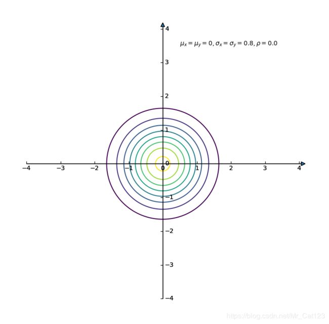
(注意:在上面的图片中,不相关的二维正太分布每个截面都是圆形,表示不相关)
即,在一元标准正太分布中,分布密度为
(2.1.1) f ( x ) = 1 2 π e − x 2 2 , − ∞ < x < ∞ , f(x)=\frac{1}{\sqrt{2\pi}}e^{-\frac{x^2}{2}}, -\infty<x<\infty, \tag{2.1.1} f(x)=2π1e−2x2,−∞<x<∞,(2.1.1)
而在 n n n元标准正太分布中,分布密度为
(2.1.2) f ( z ) = 1 ( 2 π ) n σ z e − z 2 2 , σ z = σ 1 σ 2 … σ n , f(z)=\frac{1}{\left(\sqrt{2\pi}\right)^n\sigma_z}e^{-\frac{z^2}{2}}, \sigma_z=\sigma_1\sigma_2\ldots \sigma_n,\tag{2.1.2} f(z)=(2π)nσz1e−2z2,σz=σ1σ2…σn,(2.1.2)
所以,需要记住的是,最一般的 n n n维高斯分布密度函数为
(2.1.3) f ( z ) = 1 ( 2 π ) n ∣ Σ ∣ 1 / 2 e − ( x − μ x ) T ( Σ ) − 1 ( x − μ x ) 2 , f(z)=\frac{1}{\left(\sqrt{2\pi}\right)^n|\Sigma|^{1/2}}e^{-\frac{(x-\mu_x)^T(\Sigma)^{-1}(x-\mu_x)}{2}},\tag{2.1.3} f(z)=(2π)n∣Σ∣1/21e−2(x−μx)T(Σ)−1(x−μx),(2.1.3)
( x − μ x ) T = [ ( x 1 − μ x 1 ) ( x 2 − μ x 2 ) … ] 是 行 矩 阵 (x-\mu_x)^T=[(x_1-\mu_{x_1}) (x_2-\mu_{x_2})\ldots] 是行矩阵 (x−μx)T=[(x1−μx1)(x2−μx2)…]是行矩阵
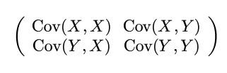
Σ 是 协 方 差 矩 阵 \Sigma是协方差矩阵 Σ是协方差矩阵以2维矩阵为例, Σ \Sigma Σ的表达式为
2.2 举例-画2维独立不相关高斯图
即上面 ( 2.1.2 ) (2.1.2) (2.1.2)的 n = 2 n=2 n=2的情况
(2.2.1) f ( x ) = 1 ( 2 π ) 2 σ 1 σ 2 e − ( x 1 − μ 1 ) 2 2 σ 1 2 − ( x 2 − μ 2 ) 2 2 σ 2 2 , f(x)=\frac{1}{\left(\sqrt{2\pi}\right)^2\sigma_1\sigma_2}e^{-\frac{(x_1-\mu_1)^2}{2\sigma_1^2}-\frac{(x_2-\mu_2)^2}{2\sigma_2^2}},\tag{2.2.1} f(x)=(2π)2σ1σ21e−2σ12(x1−μ1)2−2σ22(x2−μ2)2,(2.2.1)

import numpy as np
import matplotlib.pyplot as plt
import mpl_toolkits.axisartist as axisartist
from mpl_toolkits.mplot3d import Axes3D #画三维图不可少
from matplotlib import cm  #cm 是colormap的简写

#定义坐标轴函数
def setup_axes(fig, rect):
    ax = axisartist.Subplot(fig, rect)
    fig.add_axes(ax)

    ax.set_ylim(-.2, 1.2)
    #自定义刻度
#    ax.set_yticks([-10, 0,9])
    ax.set_xlim(-10,10)
    ax.axis[:].set_visible(False)

	#第2条线,即y轴,经过x=0的点
    ax.axis["y"] = ax.new_floating_axis(1, 0)
    ax.axis["y"].set_axisline_style("-|>", size=1.5)
#    第一条线,x轴,经过y=0的点
    ax.axis["x"] = ax.new_floating_axis(0, 0)
    ax.axis["x"].set_axisline_style("-|>", size=1.5)

    return(ax)
# 1_dimension gaussian function
def gaussian(x,mu,sigma):
    f_x = 1/(sigma*np.sqrt(2*np.pi))*np.exp(-np.power(x-mu, 2.)/(2*np.power(sigma,2.)))
    return(f_x)

# 2_dimension gaussian function
def gaussian_2(x,y,mu_x,mu_y,sigma_x,sigma_y):
    f_x_y = 1/(sigma_x*sigma_y*(np.sqrt(2*np.pi))**2)*np.exp(-np.power\
              (x-mu_x, 2.)/(2*np.power(sigma_x,2.))-np.power(y-mu_y, 2.)/\
              (2*np.power(sigma_y,2.)))
    return(f_x_y)

#设置2维表格
x_values = np.linspace(-5,5,2000)
y_values = np.linspace(-5,5,2000)
X,Y = np.meshgrid(x_values,y_values)
#高斯函数
mu_x,mu_y,sigma_x,sigma_y = 0,0,0.8,0.8
F_x_y = gaussian_2(X,Y,mu_x,mu_y,sigma_x,sigma_y)
#显示三维图
fig = plt.figure()
ax = plt.gca(projection='3d')
ax.plot_surface(X,Y,F_x_y,cmap='jet')
# 显示等高线图
#ax.contour3D(X,Y,F_x_y,50,cmap='jet')
# 显示2d等高线图,画8条线
# plt.contour(X,Y,F_x_y,8)
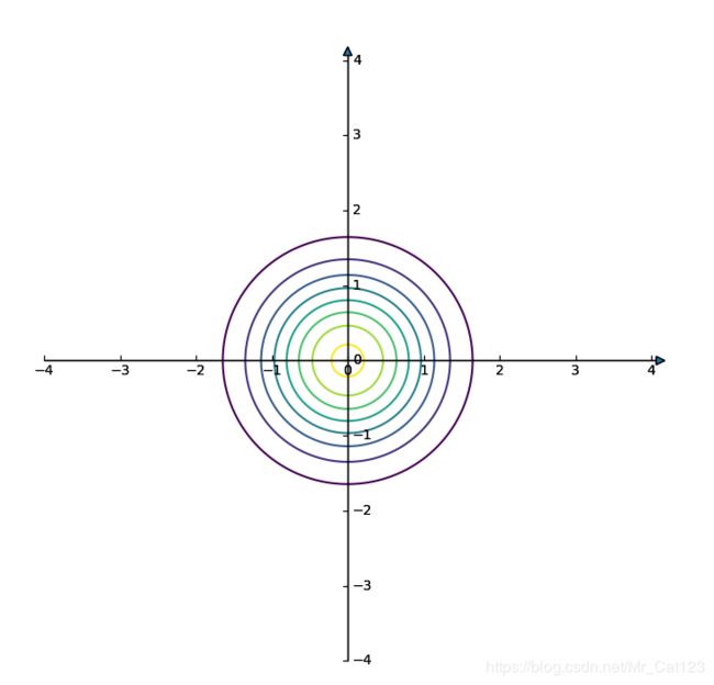
如果画成平面上的等高线图会更好理解,如下图,是一个个圆,也就是无相关
    ax.set_ylim(-4, 4)
    #自定义刻度
#    ax.set_yticks([-10, 0,9])
    ax.set_xlim(-4,4)
#设置画布
fig = plt.figure(figsize=(8, 8)) #建议可以直接plt.figure()不定义大小
ax1 = setup_axes(fig, 111)
ax1.axis["x"].set_axis_direction("bottom")
ax1.axis['y'].set_axis_direction('right')
# 显示2d等高线图,画8条线
plt.contour(X,Y,F_x_y,8)
2.3 相关系数
这里参考高数三P342.
定义:设二维随机向量 ( X , Y ) (X,Y) (X,Y)的方差 D X > 0 , D Y > 0 DX>0, DY>0 DX>0,DY>0,协方差 C o v ( X , Y ) Cov(X,Y) Cov(X,Y)都存在,则称
ρ X , Y = C o v ( X , Y ) D X D Y = C o v ( X , Y ) σ X σ Y \rho_{X,Y}=\frac{Cov(X,Y)}{\sqrt{DX}\sqrt{DY}}=\frac{Cov(X,Y)}{\sigma_X\sigma_Y} ρX,Y=DXDYCov(X,Y)=σXσYCov(X,Y)
为随机变量 X 和 Y X和Y X和Y的相关系数
性质:
- ∣ ρ X Y ∣ ≤ 1 |\rho_{XY}|\leq1 ∣ρXY∣≤1
- ρ \rho ρ是可以为负数的
- ρ 越 接 近 1 \rho越接近1 ρ越接近1表明相关程度越大, ρ = 1 \rho=1 ρ=1表明随机点 ( X , Y ) (X,Y) (X,Y)在 y = a x + b y=ax+b y=ax+b线上; ρ = 0 \rho=0 ρ=0表示不相关,此时协方差=0
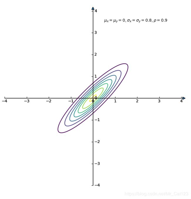
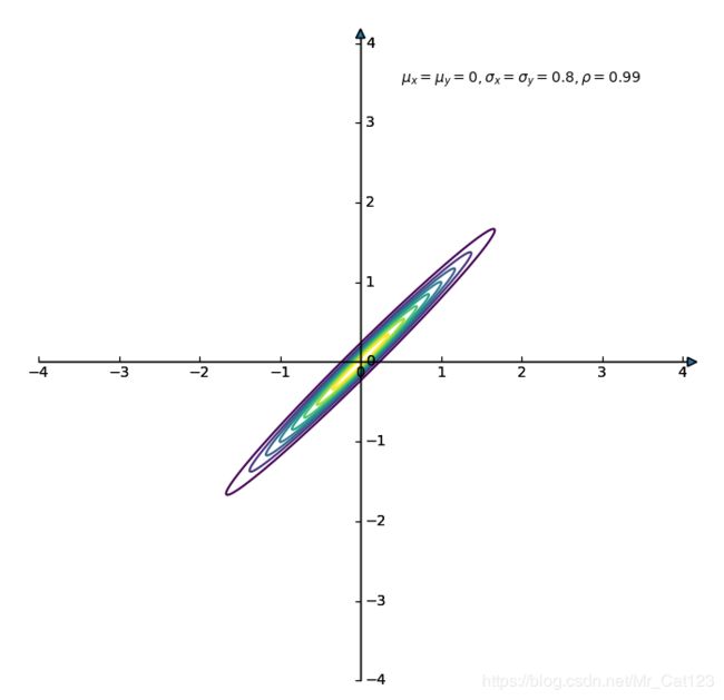
2.3 举例-画2维不独立相关高斯图
协方差矩阵 Σ \Sigma Σ的形式为 (2.3,1) \tag{2.3,1} (2.3,1)

对角线上是方差,其他是协方差,当随机变量之间不独立的时候,协方差是不为零的。上面的协方差矩阵可以写成 (2.3,2) \tag{2.3,2} (2.3,2)

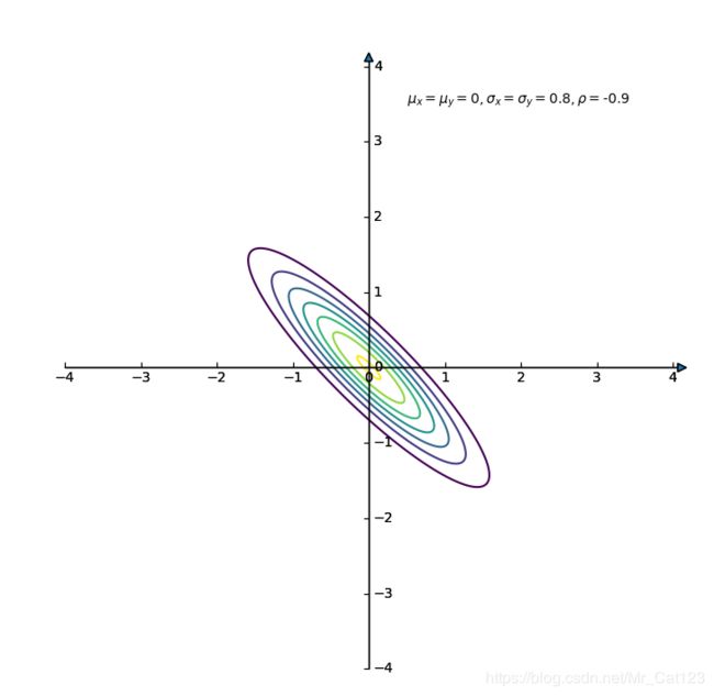
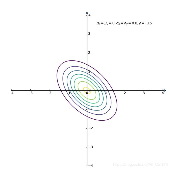
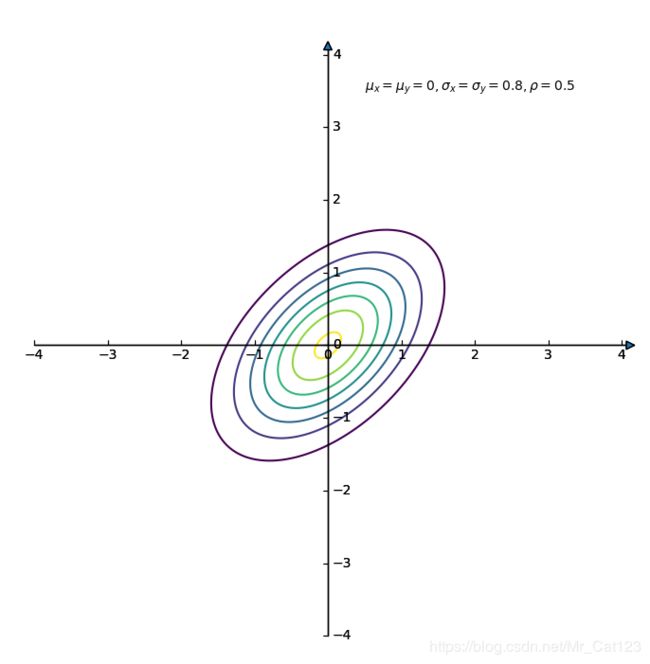
公式 ( 2.1.3 ) (2.1.3) (2.1.3)考虑相关时, ρ \rho ρ不等于0,此时协方差矩阵 Σ \Sigma Σ是 ( 2.3.2 ) (2.3.2) (2.3.2)的形式,因此分布密度函数为
(2.3.3) f ( x ) = 1 2 π σ 1 σ 2 1 − ρ 2 e − 1 2 ( 1 − ρ 2 ) [ ( x 1 − μ 1 ) 2 σ 1 2 − 2 ρ ( x − μ 1 ) ( x − μ 2 ) σ 1 σ 2 + ( x 2 − μ 2 ) 2 σ 2 2 ] f(x)=\frac{1}{2\pi\sigma_1\sigma_2\sqrt{1-\rho^2}}e^{-\frac{1}{2(1-\rho^2)}\left[\frac{(x_1-\mu_1)^2}{\sigma_1^2}-2\rho\frac{(x-\mu_1)(x-\mu_2)}{\sigma_1\sigma_2}+\frac{(x_2-\mu_2)^2}{\sigma_2^2}\right]}\tag{2.3.3} f(x)=2πσ1σ21−ρ21e−2(1−ρ2)1[σ12(x1−μ1)2−2ρσ1σ2(x−μ1)(x−μ2)+σ22(x2−μ2)2](2.3.3)
过程如下:
现在,画出2维高斯分布相关图
现在画出几种相关图,首先看一下三维图