Parzen Window and Likelihood

Kernel density estimation via the Parzen-Rosenblatt window method

Generative Adversarial Nets code

Nice explanation

对Ian提到的采用Gassian Parzen Window 去拟合G产生的样本并估计对数似然性(即给予观察样本，判断模型正确的可能性)如何实现的原理很感兴趣？
于是找到源代码parzen_ll.py来看，
但是苦于并没有学过theano及pylearn2所以看起来不是明白，本来想尝试安装py2learn来测试，结果看了官网的安装要求，请卸载python，清除所有组件。这个代价有点大
，毕竟我是要做Tensorflow的。因此只能破罐破摔来，硬着头皮看代码，有些东西只能靠google，看了一个大概。首先来说一下Parzen Window

2 Defining the Region Rn

Parzen windown 是一种应用广泛的非参数估计方法，从采样的样本 p(xn) p ( x n ) 中估计概率密度函数 p(x) p ( x ) 。
这种方法最基本的思想是给定一个特定的区域（Window）对落入其中的样本进行计数，可以得到样本落入该区域的概率大约为：

p(x)=knn p ( x ) = k n n

从数学的角度来求取在区域R里k个观察样本的概率，我们可以考虑一个Binomial(二项式分布）：

pk=[nk]⋅pk⋅(1−p)n−k p k = [ n k ] ⋅ p k ⋅ ( 1 − p ) n − k

然后在二项式分布假设的情况下， 所以我们可以求得其均值为：

E[k]=n⋅p E [ k ] = n ⋅ p

在连续性假设条件下：

p(x)=∫Rf(x)dx=f(x)⋅V p ( x ) = ∫ R f ( x ) d x = f ( x ) ⋅ V

其中v为区域R的体积，我们可以对公式进行变形，可以得到：

f(x)=p(x)V=k/nV f ( x ) = p ( x ) V = k / n V

上面简单的公式可以让计算给定点 x x 的概率密度，通过计算有多少点落入确定性区域。

确定区域的两种不同的方法

一种方法是固定体积（volume）如下图，原理是取一个固定大小的区域R，观察有多少样本落入其中。

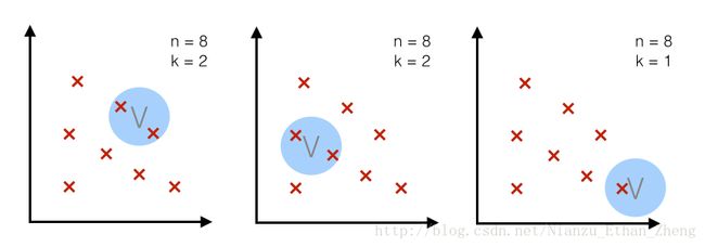
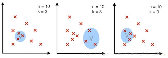
另外一种方法是样本数目K固定；k近邻算法就是这个原理，即是，对于一定大小的样本总数，我们取能框住k个样本的区域R

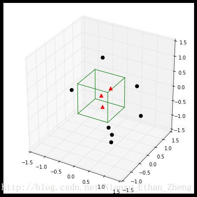
3D- hypercubes

The window function

如上面所示，我们可以可视化区域 R R ，也就很容易计算出多少点在区域内，数学表达上是：

ϕ(u)=[10|uj|≤1/2;j=1,2,...,dotherwise ϕ ( u ) = [ 1 | u j | ≤ 1 / 2 ; j = 1 , 2 , . . . , d 0 o t h e r w i s e

扩展概念（立方体核，hyercube window）我们可以得到下面的概念：
通过下面的公式可以获得落入该区域的样本个数Kn

kn=∑i=1nϕ(x−xi,hn) k n = ∑ i = 1 n ϕ ( x − x i , h n )

式中：

u=(x−xihn) u = ( x − x i h n )

也就是：

ϕ(x−xi,hn)=[10∣∣x−xihn∣∣≤1/2;j=1,2,...,dotherwise ϕ ( x − x i , h n ) = [ 1 | x − x i h n | ≤ 1 / 2 ; j = 1 , 2 , . . . , d 0 o t h e r w i s e

进而我们可以的得到Rn的概率

而将将简单的立方体核函数替换掉，采用高斯核：

ϕ(x−xi,hn)=1(2π)d/2|Σ|1/2exp(−(x−xi)TΣ−1(x−xi)2h2) ϕ ( x − x i , h n ) = 1 ( 2 π ) d / 2 | Σ | 1 / 2 exp ⁡ ( − ( x − x i ) T Σ − 1 ( x − x i ) 2 h 2 )

Parzen window estimation

基于上述公式，我们可以得到：

pn(x)=1n∑i=1n1hdϕ[x−xi,hn] p n ( x ) = 1 n ∑ i = 1 n 1 h d ϕ [ x − x i , h n ]

式中有：

Vn=hd V n = h d

k=∑i=1nϕ[x−xi,hn] k = ∑ i = 1 n ϕ [ x − x i , h n ]

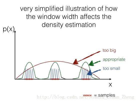
Parzen-window技术的关键性参数

这有两个关键性参数：
- 核函数（kernel function）
- 核宽度（window width）

核密度估计需要满足如下条件：
1） 有限值非负密度函数：

∫f(y,h)dy=1 ∫ f ( y , h ) d y = 1

2） 对于核宽度的要求

limn→∞nhd(n)=∞ lim n → ∞ ⁡ n h d ( n ) = ∞

limn→∞hd=0 lim n → ∞ ⁡ h d = 0

limn→∞kn=∞ lim n → ∞ ⁡ k n = ∞

一式原因在于：

limn→∞pn(x)=p(x) lim n → ∞ ⁡ p n ( x ) = p ( x )

limn→∞knn⋅V=p(x) lim n → ∞ ⁡ k n n ⋅ V = p ( x )

构造Parzen window估计函数

def parzen_estimation(mu, sigma, mode='gauss'):
    """
    Implementation of a parzen-window estimation
    Keyword arguments:
        x: A "nxd"-dimentional numpy array, which each sample is
                  stored in a separate row (=training example)
        mu: point x for density estimation, "dx1"-dimensional numpy array
        sigma: window width
    Return the density estimate p(x)
    """

    def log_mean_exp(a):
        max_ = a.max(axis=1)
        return max_ + np.log(np.exp(a - np.expand_dims(max_, axis=0)).mean(1))

    def gaussian_window(x, mu, sigma):
        a = (np.expand_dims(x, axis=1) - np.expand_dims(mu, axis=0)) / sigma
        b = np.sum(- 0.5 * (a ** 2), axis=-1)
        E = log_mean_exp(b)
        Z = mu.shape[1] * np.log(sigma * np.sqrt(np.pi * 2))
        return np.exp(E - Z)

    def hypercube_kernel(x, mu, h):
        n, d = mu.shape
        a = (np.expand_dims(x, axis=1) - np.expand_dims(mu, axis=0)) / h
        b = np.all(np.less(np.abs(a), 1/2), axis=-1)
        kn = np.sum(b.astype(int), axis=-1)
        return kn / (n * h**d)

    if mode is 'gauss':
        return lambda x: gaussian_window(x, mu, sigma)
    elif mode is 'hypercube':
        return lambda x: hypercube_kernel(x, mu, h=sigma)

将Parzen Window 方法应用于高斯数据集

我们构造如下数据集：

f(x)=1(2π)d/2|Σ|1/2exp(−(x−xi)TΣ−1(x−xi)2) f ( x ) = 1 ( 2 π ) d / 2 | Σ | 1 / 2 exp ⁡ ( − ( x − x i ) T Σ − 1 ( x − x i ) 2 )

设定：

u=[00]Σ=[1001] u = [ 0 0 ] Σ = [ 1 0 0 1 ]

import numpy as np

# Generate 10,000 random 2D-patterns
mu_vec = np.array([0,0])
cov_mat = np.array([[1,0],[0,1]])
x_2Dgauss = np.random.multivariate_normal(mu_vec, cov_mat, 10000)

print(x_2Dgauss.shape)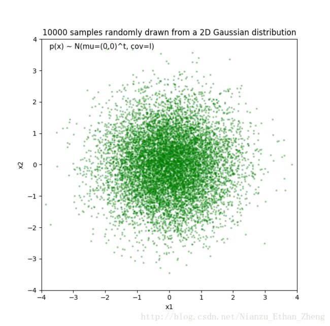

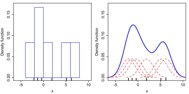
不同核函数对于pdf的估计效果不同

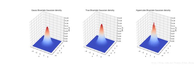
可以看到高斯核函数的概率密度估计过渡更加自然，而超维度的高斯估计则虽然相比较精度较高一些但是毛刺比较严重。

模型	[0, 0]
真实值	0.15915494309189535
hypercube（h=0.3）	0.15444444
Gauss(h=0.3)	0.14109129

import matplotlib.pyplot as plt
    from mpl_toolkits.mplot3d import Axes3D
    from matplotlib import cm
    from matplotlib.ticker import LinearLocator, FormatStrFormatter

    # Make data
    mu_vec = np.array([0, 0])
    cov_mat = np.array([[1, 0], [0, 1]])
    x_2Dgauss = np.random.multivariate_normal(mu_vec, cov_mat, 10000)

    # Pdf estimation
    def pdf_multivaraible_gauss(x, mu, cov):
        part1 = 1 / ((2 * np.pi) ** (len(mu)/2) * (np.linalg.det(cov)**(1/2)))
        part2 = (-1/2) * (x-mu).T.dot(np.linalg.inv(cov)).dot((x-mu))
        return float(part1 * np.exp(part2))

    ph = parzen_estimation(x_2Dgauss, 0.3, mode='hypercube')
    pg = parzen_estimation(x_2Dgauss, 0.3, mode='gauss')
    print(pdf_multivaraible_gauss(np.array([[0], [0]]), np.array([[0], [0]]), cov_mat))
    print(ph([[0, 0]]))
    print(pg([[0, 0]]))

    x = np.linspace(-5, 5, 100)
    x, y = np.meshgrid(x, x)
    zg = []
    zt = []
    zh = []
    for i, j in zip(x.ravel(), y.ravel()):
        zg.append(pg([[i, j]]))
        zh.append(ph([[i, j]]))
        zt.append(pdf_multivaraible_gauss(np.array([[i], [j]]), np.array([[0], [1]]), cov_mat))
    zg = np.asarray(zg).reshape(100, 100)
    zh = np.asarray(zh).reshape(100, 100)
    zt = np.asarray(zt).reshape(100, 100)

    # Plot the surface
    fig = plt.figure(figsize=(18, 6))
    ax1 = fig.add_subplot(131, projection='3d')
    surf = ax1.plot_surface(x, y, zg, rstride=1, cstride=1,
                            cmap=cm.coolwarm, antialiased=False)
    # Customize the z axis
    ax1.zaxis.set_major_locator(LinearLocator(10))
    ax1.zaxis.set_major_formatter(FormatStrFormatter('%.02f'))
    ax1.set(zlim=[0, 0.2], xlabel='x', ylabel='y', zlabel='p(x,y)',
            title="Gauss Bivariate Gaussian density")

    # Re-Plot
    ax2 = fig.add_subplot(132, projection='3d')
    ax2.plot_surface(x, y, zt, rstride=1, cstride=1, cmap=cm.coolwarm, antialiased=False)

    # Customize the z axis
    ax2.zaxis.set_major_locator(LinearLocator(10))
    ax2.zaxis.set_major_formatter(FormatStrFormatter('%.02f'))
    ax2.set(zlim=[0, 0.2], xlabel='x', ylabel='y', zlabel='p(x,y)',
            title="True Bivariate Gaussian density")

    # Re-Plot
    ax3 = fig.add_subplot(133, projection='3d')
    ax3.plot_surface(x, y, zh, rstride=1, cstride=1, cmap=cm.coolwarm, antialiased=False)

    # Customize the z axis
    ax3.zaxis.set_major_locator(LinearLocator(10))
    ax3.zaxis.set_major_formatter(FormatStrFormatter('%.02f'))
    ax3.set(zlim=[0, 0.2], xlabel='x', ylabel='y', zlabel='p(x,y)',
            title="Hypercube Bivariate Gaussian density")

    # Add a color bar which maps values to colors.
    fig.savefig("./Gauss_kernel_{}.png".format('Bivariate_Gaussian'))
    plt.show()

不同核宽度对pdf估计的影响

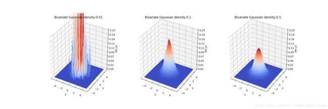
可以看到当核宽度非常小（0.01）时， pdf已经不可控， 而当h=0.5, 估计效果又有所下降。因此如何能根据数据样本来确定核宽度大小，是一个非常重要的问题。

    import matplotlib.pyplot as plt
    from mpl_toolkits.mplot3d import Axes3D
    from matplotlib import cm
    from matplotlib.ticker import LinearLocator, FormatStrFormatter

    # Make data
    mu_vec = np.array([0, 0])
    cov_mat = np.array([[1, 0], [0, 1]])
    x_2Dgauss = np.random.multivariate_normal(mu_vec, cov_mat, 10000)

    # Pdf estimation
    def pdf_multivaraible_gauss(x, mu, cov):
        part1 = 1 / ((2 * np.pi) ** (len(mu)/2) * (np.linalg.det(cov)**(1/2)))
        part2 = (-1/2) * (x-mu).T.dot(np.linalg.inv(cov)).dot((x-mu))
        return float(part1 * np.exp(part2))

    pg1 = parzen_estimation(x_2Dgauss, 0.01, mode='gauss')
    pg2 = parzen_estimation(x_2Dgauss, 0.1, mode='gauss')
    pg3 = parzen_estimation(x_2Dgauss, 0.5, mode='gauss')
    x = np.linspace(-5, 5, 100)
    x, y = np.meshgrid(x, x)
    zg = []
    zh = []
    zt = []
    for i, j in zip(x.ravel(), y.ravel()):
        zg.append(pg1([[i, j]]))
        zh.append(pg2([[i, j]]))
        zt.append(pg3([[i, j]]))
    zg = np.asarray(zg).reshape(100, 100)
    zh = np.asarray(zh).reshape(100, 100)
    zt = np.asarray(zt).reshape(100, 100)

    # Plot the surface
    fig = plt.figure(figsize=(18, 6))
    ax1 = fig.add_subplot(131, projection='3d')
    surf = ax1.plot_surface(x, y, zg, rstride=1, cstride=1,
                            cmap=cm.coolwarm, antialiased=False)
    # Customize the z axis
    ax1.zaxis.set_major_locator(LinearLocator(10))
    ax1.zaxis.set_major_formatter(FormatStrFormatter('%.02f'))
    ax1.set(zlim=[0, 0.2], xlabel='x', ylabel='y', zlabel='p(x,y)',
            title="Bivariate Gaussian density-0.01")

    # Re-Plot
    ax2 = fig.add_subplot(132, projection='3d')
    ax2.plot_surface(x, y, zh, rstride=1, cstride=1, cmap=cm.coolwarm, antialiased=False)

    # Customize the z axis
    ax2.zaxis.set_major_locator(LinearLocator(10))
    ax2.zaxis.set_major_formatter(FormatStrFormatter('%.02f'))
    ax2.set(zlim=[0, 0.2], xlabel='x', ylabel='y', zlabel='p(x,y)',
            title="Bivariate Gaussian density-0.1")

    # Re-Plot
    ax3 = fig.add_subplot(133, projection='3d')
    ax3.plot_surface(x, y, zt, rstride=1, cstride=1, cmap=cm.coolwarm, antialiased=False)

    # Customize the z axis
    ax3.zaxis.set_major_locator(LinearLocator(10))
    ax3.zaxis.set_major_formatter(FormatStrFormatter('%.02f'))
    ax3.set(zlim=[0, 0.2], xlabel='x', ylabel='y', zlabel='p(x,y)',
            title="Bivariate Gaussian density-0.5")

    # Add a color bar which maps values to colors.
    fig.savefig("./Gauss_kernel_{}.png".format('Gauss_width'))
    plt.show()

已知真实分布情况下

我们可以计算出最好的核宽度为，通过误差图来观察

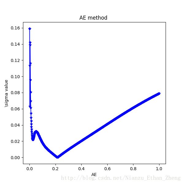
可以看到 h = 0.21529369369369367

当然大多数情况下并不知道真实的概率分布，那可以通过最大似然法来选择核宽度

首先介绍似然性

Likelihood

可能性其实就是所有采的样本在你所建立的模型中概率的乘积，让这个乘积最大就是最大似然法，而为了计算方便，采用对数的方法，将
乘积运算转换为加法运算。

对parzen_ll的理解

终于到了主题：

def theano_parzen(mu, sigma):
    """
    Credit: Yann N. Dauphin
    """

    x = T.matrix()
    mu = theano.shared(mu)
    a = ( x.dimshuffle(0, 'x', 1) - mu.dimshuffle('x', 0, 1) ) / sigma
    E = log_mean_exp(-0.5*(a**2).sum(2))
    Z = mu.shape[1] * T.log(sigma * numpy.sqrt(numpy.pi * 2))

    return theano.function([x], E - Z)

这个函数用于创造一个parzen的计算器，其中x的大小为2D向量，通过dimshuffule来变为Ax1xB 这样的向量，mu为图像的所有像素的值，sigma对于所有维都是固定的均为sigma。通过创造一个log_mean_exp函数计算平均值

def log_mean_exp(a):
    """
    Credit: Yann N. Dauphin
    """

    max_ = a.max(1)

    return max_ + T.log(T.exp(a - max_.dimshuffle(0, 'x')).mean(1))

定义好Parzen函数之后，通过get_nll函数获得似然值，其中的操作是每次输入一个batch_size,最后对各个batch_size求取平均值

def get_nll(x, parzen, batch_size=10):
    """
    Credit: Yann N. Dauphin
    """

    inds = range(x.shape[0])
    n_batches = int(numpy.ceil(float(len(inds)) / batch_size))

    times = []
    nlls = []
    for i in range(n_batches):
        begin = time.time()
        nll = parzen(x[inds[i::n_batches]])
        end = time.time()
        times.append(end-begin)
        nlls.extend(nll)

        if i % 10 == 0:
            print i, numpy.mean(times), numpy.mean(nlls)

    return numpy.array(nlls)

其中可以追查mu的来源,mu ==samples ,于是在下面我们可以发现出mu的蛛丝马迹，reshape函数将三个通道的图片扁平为一维向量，而整个空间定格为整个图片的像素点数。

samples = model.generator.sample(args.num_samples).eval()
    output_space = model.generator.mlp.get_output_space()
    if 'Conv2D' in str(output_space):
        samples = output_space.convert(samples, output_space.axes, ('b', 0, 1, 'c'))
        samples = samples.reshape((samples.shape[0], numpy.prod(samples.shape[1:])))
    del model
    gc.collect()

值得一提的是为了获得较好的估计值，他采用验证集来确定最大的似然值对应的sigma,验证集采用的是50000-60000的MNIST字体。

def cross_validate_sigma(samples, data, sigmas, batch_size):

    lls = []
    for sigma in sigmas:
        print sigma
        parzen = theano_parzen(samples, sigma)
        tmp = get_nll(data, parzen, batch_size = batch_size)
        lls.append(numpy.asarray(tmp).mean())
        del parzen
        gc.collect()

    ind = numpy.argmax(lls)
    return sigmas[ind]

Parzen Window的公式大致对的上，明确了输入（对于MNIST）是60000x1x784的一个批次，大约10个，主要可能考虑到对于高达784的多变量高斯分布计算量必然很大。
然后考虑到likelihood的计算公式

将Parzen Window估计概率并应用于求解最大似然法，目前来说，对求解似然性于不是最好的办法，但是也没有更好的办法。其基本思路大致是，产生的样本通过高斯核Parzen窗口法计算出一个概率模型Pg（784维的高斯分布），然后估计测试样本的概率，从而计算出在该分布下的对数似然性，方差参数采用交叉验证来获得。

最大似然法

import matplotlib.pyplot as plt
    from mpl_toolkits.mplot3d import Axes3D
    from matplotlib import cm
    from matplotlib.ticker import LinearLocator, FormatStrFormatter

    # Make data
    np.random.seed(2017)
    mu_vec = np.array([0, 0])
    cov_mat = np.array([[1, 0], [0, 1]])
    x_2Dgauss = np.random.multivariate_normal(mu_vec, cov_mat, 10000)
    x_test = np.random.multivariate_normal(mu_vec, cov_mat, 1000)

    pg = parzen_estimation(x_2Dgauss, 0.01, mode='gauss')
    sigma, nll = cross_validate_sigma(x_2Dgauss, x_test, np.linspace(1e-4, 1, 20), batch_size=100)
    fig = plt.figure(figsize=(6, 6))
    ax = fig.gca()
    ax.plot(np.linspace(1e-4, 1, 20), nll,  '-*r')
    ax.set(xlabel='log likelihood', ylabel='\sigma value', title='NLL method ')
    print(sigma)
    fig.savefig('./{}.png'.format('NLL_method'))
    plt.show()
    # Pdf estimation
    def pdf_multivaraible_gauss(x, mu, cov):
        part1 = 1 / ((2 * np.pi) ** (len(mu)/2) * (np.linalg.det(cov)**(1/2)))
        part2 = (-1/2) * (x-mu).T.dot(np.linalg.inv(cov)).dot((x-mu))
        return float(part1 * np.exp(part2))


    tr = pdf_multivaraible_gauss(np.array([[0], [0]]), np.array([[0], [0]]), cov_mat)
    errs = []
    sigmas = np.linspace(1e-4, 1, 1000)
    for sigma in sigmas:
        pg = parzen_estimation(x_2Dgauss, sigma, mode='gauss')
        err = np.abs(pg(np.array([[0, 0]]))-tr)
        errs.append(err)
    fig = plt.figure(figsize=(6, 6))
    ax = fig.gca()
    ax.plot(sigmas, errs, '-*b')
    ax.set(xlabel='AE', ylabel='\sigma value', title='AE method ')
    ind = np.argmin(errs)
    print(sigmas[ind])
    fig.savefig('./{}.png'.format('AE_method'))
    plt.show()

可以看到在h = 0.21060526315789474， 附近似然性取得最大值

方法	最优值
最大似然法	0.21060526315789474
误差法	0.21529369369369367

可以看到极大似然法可以有效估计核宽度。

Parzen window 技术的优缺点：

Parzen window技术作为一种非参数方法，有着和其他方法一样的缺点，就是每次估计需要整个样本参与运算，而并非是参数估计，只是带入参数计算。
几个挑战：
1） 数据样本的大小， Parzen window的计算复杂度为 n2d n 2 d , 其中 n n 为训练样本数目， 而 d d 为样本维度。

2） 合适的核宽度的选择， 一般来说：

hn∝1n−−√ h n ∝ 1 n

hn∝1log（n） h n ∝ 1 l o g （ n ）

3) 核函数的选择

4) 应用于两个方面：Bayes估计与互信息的求取