【Faster RCNN】Faster R-CNN笔记

论文理论笔记部分：

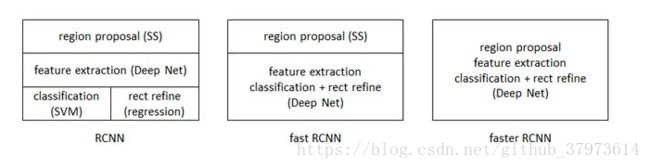
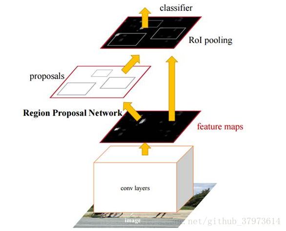
rcnn是将每个proposal都放入到卷积层来进行计算，fast rcnn呢，则是将图片和proposal作为输入，并且proposal是为feature map的提取提供位置信息、为regression提供位置信息、以及在classification提供位置信息。在这里，faster rcnn的输入是一张图，提取到了共享的feature map后，将feature map用来进行RPN提取proposals操作以及联合RPN的输出进行ROIs操作，最后作为fast rcnn网络的输入来做回归和分类。

图片来源

 

Two modules:

• a deep fully convolution network that proposes regions as an attention mechanism.
• the fast RCNN detector that uses the proposed regions.

faster RCNN

1、RPN（Region Proposal Networks）

sppnet和fast RCNN减少了检测网络的时间，但是region proposal还是耗费很多时间。FASTER-RCNN解决了这个问题，提出了Region Proposal Network（RPN）代替selective search部分。

输入：image with any size；

输出：rectangular obect proposals with objectness score。

ultimate goal: share computation with a Fast R-CNN，implement end-to-end network.

 

Fast RCNN结构图

为了使RPN和fast rcnn分享卷积特征，所以这两个网络要使用同样的卷积层。在论文中，使用了ZF和VGG19两个网络的卷积层，作为共享卷积层。

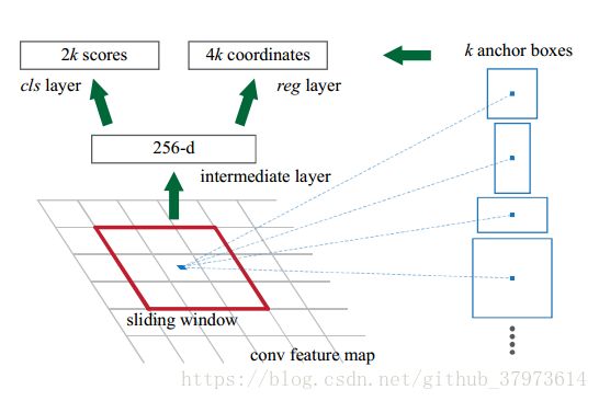
如上图所示，为了生成region proposals，在最后一个卷积层上，用一个n*n（n=3）的小窗口（卷积层）滑动每个位置，把特征降为256维。把这256为特征分别输入到连个全连接层cls和reg。

 

2、Translation-Invariant Anchors（平移不变性）：

如果移动了一张图像中的一个物体，这proposal应该也移动了，而且相同的函数可以预测出热议未知的proposal。MultiBox不具备如此功能。平移不变性可以介绍模型大小。

在每个滑动窗口的位置预测k个region proposal（实验默认k=9）叫做anchor，默认使用3种尺度（scale:实验中使用128^2，256^2，512^2）和3种长宽比（ratio：实验中使用1：1，1：2，2：1），以滑动窗口的中心点为中心（An anchor is centered at the sliding window in question.）。对于一个convolutional feature map of size ，一共有个anchor（这里因为每个窗口点产生一个feature map 单元，每个单元里有k个anchors）。

【our anchor-based method is built on a pyramind of anchors, which is more cost-efficient.Our method classifies and regresses bounding boxes with reference to anchor boxes of multiple scales and aspect ratios】

3、Multi-Scale Anchor as Regression Reference

Two popular ways for multi-scale predictions

• based on image/feature pyramids,如DPM and CNN-based methods。图像被resized成不同尺寸，然后为每一种尺寸计算feature maps(HOG或者deep convolutional features)。这种方法比较费时。
• use sliding windows of multiple scales(and/or aspect ratio) on the feature maps——filters金字塔。第二种方法经常和第一种方法一起使用。

在本论文中：anchor金字塔——more cost-efficient，只依靠单尺寸的图像和feature map。

the design of multiscale anchors is a key component for sharing features without extra cost for addressing scales.

4、Loss Function for learning region proposal

为了训练PRNs，赋予anchors二值的类标对应是否包含object（只是是否包含有对象，不分类）。来对anchors赋label：

• positive label：
  • the anchor/anchors with the highest  IOU overlap with a ground-truth box,
  • or，an anchor that has an IOU overlap higher than 0.7 with any group-truth box.
• negative label:

           IOU ratio < 0.3 for all groud-truth boxes.

•  其余的非P非N的anchors have no contribution.

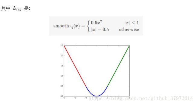
损失函数【是log loss，是smooth_L1 loss】：

tips：

is the index of an anchor

 is the predicted probability of anchor i being an object.

 为真实值 1 or 0

 是预测边界框四个坐标组成的向量

normalized by ，weighted by a balanced parameter .【在论文实验代码中：，~】

for bounding box：

，

，

，

，

tips：——>predicted box, ——>anchor box,——>groud-truth box。x与y是box的中心坐标，w，h为宽和高。

可以认为是从anchor box回归到附近的gound truth box。

5、Training RPNs

• image-centric sampling strategy
• mini-batch arises from a single image that contains many positive and negative example anchors.
• 随机在一张图片中采样256个anchors来计算一个mini-batch的loss function。正负anchors=1:1
• all new layers的权值初始化：高斯分布(, ), all other layers（比如共享卷积层）用imageNet来权值初始化。用ZF net来进行微调。
• 学习率：0.001(60k)——>0.0001(20k)
• 动量(momentum)：0.9
• weight decay：0.0005

6、Sharing Feature for RPN and Fast R-CNN

• sharing convolutional layers between the two networks, rather than learning two separate networks
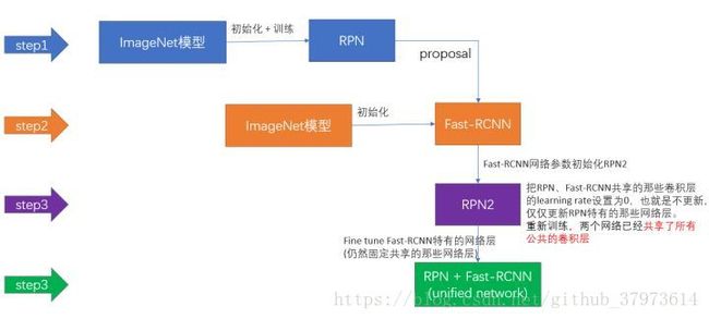
• 三种训练的方法：​​​​​
  • （1）Alternative training：迭代，先训练RPN，然后用RPN的网络权重对Fast-rcnn网络进行初始化，并用之前RPN输出的proposal去作为输入去训练Fast R-CNN。被Fast R-CNN微调的网络然后用来初始化RPN，以此迭代。本论文所有的实现都是用该方法。
  • （2）Approximate joint training：RPN和fast R-CNN融合到一个网络中进行训练。这里会有一个小瑕疵，就是会忽略掉RPN部分位置回归在反向传播时候的导数(end2end,代码常用实现)。即在下面结构中的rpn_bbox_pred-------------->proposal时，在反向传播时会切断这条路的计算，因为不方便求出其值，所以直接被忽略掉。（某一份代码里的做法）
  •                           

                                        

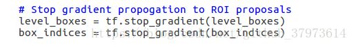
• • （3）Non-Approximate joint training：解决第二种的瑕疵，但是paper中没有提到。
  • （4）four-step Alternating Training
• 4-step Alternating Traing【作者发布的源代码】
  • step1:train RPN, initialized with an ImgNet-pre-trained model and fine-tuned end-to-end for the region tack.
  • step2:train a separate detection network by Fast R-CNN using the proposals generated by the step1 RPN. This network is also initialized by the ImgNet-pre-trained model.At this point, the two network do not share conv layers.
  • step3:use the detector network to initialize RPN training, but we fix the shared conv layers and only fine-tuned the layers unique to RPN. Now the two networks share conv layers.
  • step4:keep the shared conv layers fixed, fine-tune the unique layers of Fast R-CNN.

 

7、implementation Details

• Multi-scale and speed-accuracy之间的trade-off
• To reduce redundancy, we adopt non-maximun-suppression(NMS) on the proposal regions based on their cls scores.

8、网络结构（1）

（1）VGG介绍：

VGG-16:VGG名字来自于在ImageNet ILSVRC 2014竞赛中使用此网络的小组组名，首次发布于论文[Very Deep Convolution Networks for large-Scale Image Recognition]。

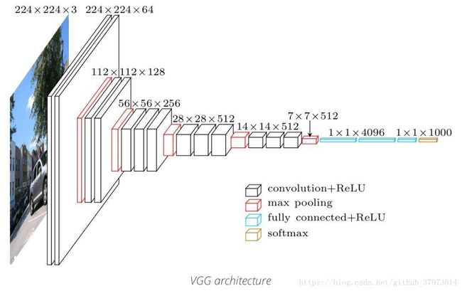
• 当使用VGG作为分类任务时，其输入是224x224x3的张量，在分裂任务中输入图片尺寸固定，因为网络最后一部分的全连接层需要固定长度的输入。在接入全连接层时，通常需要将最后一层卷积的输出展开成一维张量。
• 因为要使用卷积网络中间层的输出所以输入图片的尺寸不再有限制。因为只有卷积层参与计算。
• 每一层卷积网络都在前一层的基础上提取了更加抽象的特征。第一层学习到了简单的边缘，第二层寻找目标边缘的模式，以激活后续卷积网络中更加复杂的形状。最终，我们得到了一个在空间维度上比原始图片小很多，但表征更加深的卷积特征图。特征图的长和宽会随着卷积层间的池化二缩小，深度会随着卷积层过滤器的数量而增加。

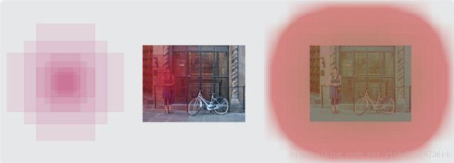
左侧：锚点， 中心：特征图空间单一锚点在原图中的表达， 右侧：所有锚点在原图中的表达

（2）RPN

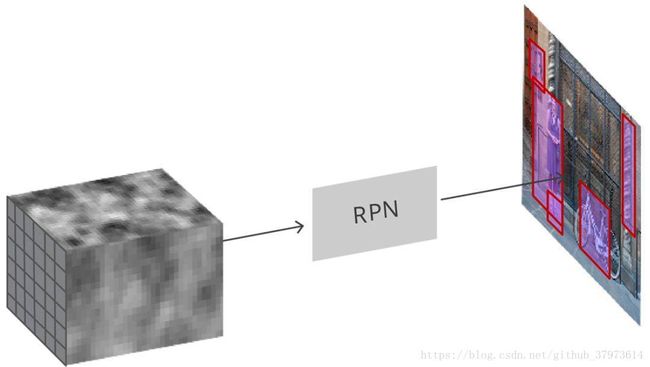
RPN采用卷积特征图并在图像上生成proposal。

• RPN接受所有的参考框（锚点）并为目标输出一套好的建议。RPN会：(i)输出锚点作为目标的概率，但是它不关心分类（2）：输出边框回归，用来调整锚点以更好的拟合其预测的目标。
• RPN是用完全卷积的方式实现的，用基础网络返回的卷积特征图作为输入。首先，我们使用一个有256个通道和3x3卷积核大小的卷积层，然后我们有两个使用1x1卷积核并行卷积网络，其通道数量取决于每个点的锚点数量。

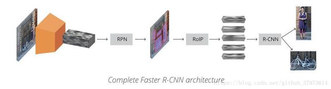
基于区域的卷积神经网络（R-CNN）是Faster R-CNN工作流的最后一步。从图像上获得卷积特征图之后，用它通过RPN来获得目标建议并最终为每个建议提取特征(通过RoI Pooling），最后我们需要使用这些特征进行分类。R-CNN试图模仿分类CNNs的最后阶段，在这个阶段用一个全连接层为每个目标类输出一个分数。

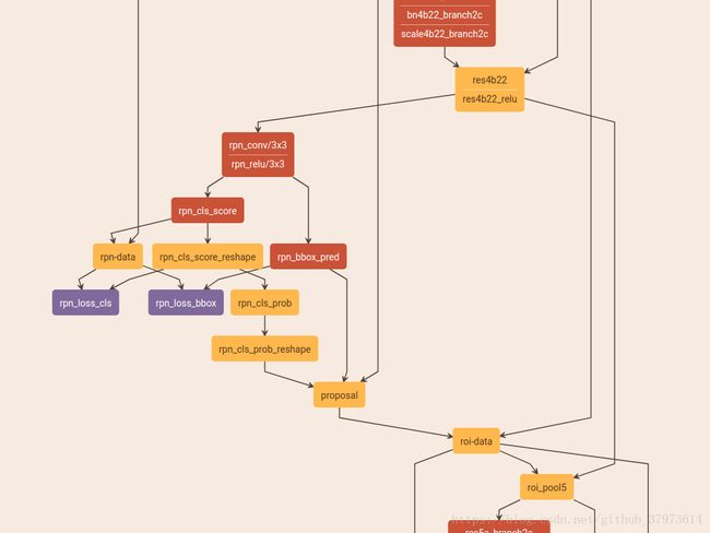
9. 网络结构（2）：参考自http://huchaowei.com/2018/01/16/faster-rcnn%E7%BD%91%E7%BB%9C%E5%89%96%E6%9E%90/

faster R-CNN=特征提取+RPN+fast R-CNN组成，这里选择ZF(VGG16)为作为特征提取的网络，再介入RPN，生成proposals。

四个部分：

• Conv layers：使用你一组基础的conv+relu+pooling层提取image的feature maps
• Region Proposal Networks（RPN）：该层生成一系列anchors并映射到原图，然后通过softmax判断anchors属于foreground或者background，再利用bounding box regression修正anchors获得精确的proposals.
• Roi Pooling：该层收集输入的feature maps和proposals，综合这些信息后提取proposal feature，送入后续全连接层判定目标类别。
• Classification和bbox regression：利用proposal feature maps计算proposal的类别，同时再次bounding box regression获取检测框最终的精确位置。

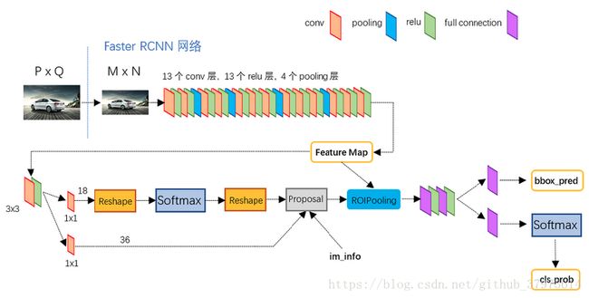
如上图：

• Conv layers：conv layers部分共分为13个conv层，13个relu层，4个pooling层。为了保证Con layers生成的feature map都可以和原图对应起来，卷积过程中使用pad保证卷积后宽高不变，经过一次pooling操作，宽高变为原来的1/2，一个MxN大小的矩阵经过conv layers固定变为(M/16)x(N/16)。一共有四次pooling，故一共是1/16。在feature后的3x3卷积，有256个通道。

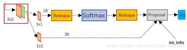
RPN

• RPN：网络分为两条线，上面的一条通过softmax分类anchors获得foreground和background（检测目标是foreground），下面一条用于计算对于anchors的bounding box regression偏移量，以获得精确的proposal。（一条分类一条回归，分类是有无目标的分类）最后的Proposal层则负责综合foreground和bounding box regression偏移量获取proposals，同时剔除大小和超出边界的proposals。
• ROI pooling层负责收集proposal，统一proposals的尺度，送入后续网络。它有两个输入：原始的proposal boxes（大小各有不同）以及原始的feature maps
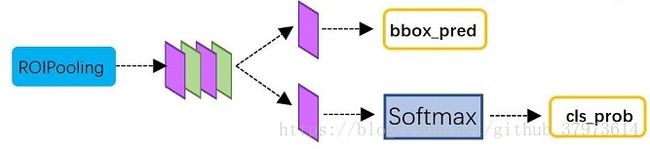
• classification：classification部分利用已经获取的Proposal feature maps，通过full connect层与softmax计算每个proposal具体属于哪个类别，输出cls_prob概率向量，同时再次利用bounding box regression获取每个proposal的位置偏移量bbox_pred，用于回归更加精确的目标检测框。
  • 通过全连接层和softmax对proposal进行分类，这实际上已经是识别的范畴了。
  • 再次对Proposal进行bounding box regression，以获取更高精度的rect box。

 

Faster R-CNN训练：

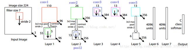ZF网络结构图（bone net）

faster R-CNN是在已经训练好的model（如VGG_CNN_M_1024, VGG, ZF）的基础上进行训练。实际训练分为6个步骤：

• 在已经训练好的model上，训练RPN网络，对应stage1_rpn_train.pt
• 利用第一步训练好的RPN，收集proposals，对应rpn_test_pt
• 第一次训练Faster RCNN网络，对应stage1_fast_rcnn_train.pt
• 第二次训练RPN网络，对应stage2_rpn_train.pt
• 再次利用第四步训练好的RPN，手机proposals，对应rpn_test.pt
• 第二次训练Fast R-CNN，对应stage2_fast_cnn_train.pt

可以看到训练的过程是一个”迭代“的过程，不过只是两次，两次的原因是：A similar alternative training can be run for more iterations. but we have observed negligible improvements。即更多了没什么效果提升。

 

 

一些细节【推荐】：

• 提取特征是与训练好的模型提取图片的特征。论文中主要使用的是caffe的预训练模型VGG16。最后提取出feature map出来。
• RPN：
  • 作者使用RPN，产生anchor是通过对每个feature map中的点都使用3种scale和3种ratio的排列组合共九种anchor。然后用这九种anchor在feature map左右上下移动，如：对一个512x62x37的feature map，有62x37x9=20000个anchor。也就是对一张图片，有20000个左右的anchor。
  • anchor的数量和feature map的数量有关，不同的feature map对应的anchor数量也不一样。RPN在CNN提取feature map的基础上，再增加一个卷积，然后利用两个1x1的卷积分别进行二分类和位置回归。进行分类的卷积核通道数量为9x2（9个anchor，每个anchor二分类，使用交叉熵损失=-yloga-(1-y)log(1-a)  ），进行回归的卷积核通道数为9x4（9个anchor，每个anchor有四个位置）。RPN是一个全卷积网络，这样对输入图片的尺寸没有要求。
  • 接下来要做的就是将20000多个候选的anchor选出256个anchor来进行分类和位置回归。选择过程前面有讲到。对于每个anchor，要么为1（前景），要么为0（背景），而gt_loc则是由四个位置参数（tx, ty, tw, th）组成，按照上面的回归公式比直接回归坐标更好。计算分类损失用的是交叉熵损失，而计算回归损失用的是Smooth_l1_loss。在计算回归损失的时候，只计算正样本（前景）的损失，不计算负样本的损失。
  • 现在利用RPN可以从上万个anchor中寻找到一定数目更有可能的候选框。在训练RCNN时，这个数目是2000，在测试推理阶段，这个数目是300（为了速度），ROI不是单纯的从anchor中选取一些出来作为候选框，它还会利用回归参数，微调anchor的形状和位置。可以这么理解：在RPN阶段，先通过feature map生成成千上万个anchor，然后利用ground truth Bounding boxes，训练这些anchor，而后从anchor中找出一定数目的候选区域（RoIs），RoIs在下一个阶段用来训练RoIHead，最后生成Predict Bounding Boxes。
• 虽然原始论文中使用4-Step Alternating Training，即四步交替迭代训练，然而现在在GitHub上，大多是采用的近似联合训练（Approximate Joint training），端到端，速度更快。那么Approximate Joint training是通过将RPN分类损失、回归损失、RoI分类损失、回归损失相加来作为最后的损失，来进行反向训练。
• 源码中的三个creator
  • AnchorTargetCreator：负责在训练RPN的时候，从上万个anchor中选择一些（比如256）进行训练，以使的正负样本的比例大概是1：1，同时给出训练的位置参数目标。即返回gt_rpn_loc和gt_rpn_label。
  • ProposalTargetCreator：负责在训练RoIHead/Fast RCNN的时候，从RoIs选择 一部分（比如128）用以训练。同时给定训练目标，返回（sample_RoI，gt_RoI_loc，gt_RoI_label）
  • ProposalCreator：在RPN中，从上万个anchor中，选择一定数目（2000或者300），调整大小和位置，生成RoIs，用以Fast RCNN训练或者测试。
  • sum：其中AnchorTargetCreator和ProposalTargetCreator是为了生成训练的目标，只是在训练阶段用到，ProposalCreator是RPN为Fast RCNN生成RoIs，在训练和测试阶段都会用到。三个共同点在于他们都不用考虑反向传播。
• 为什么在RPN的时候选择IoU阈值为0.7？
  • #pass

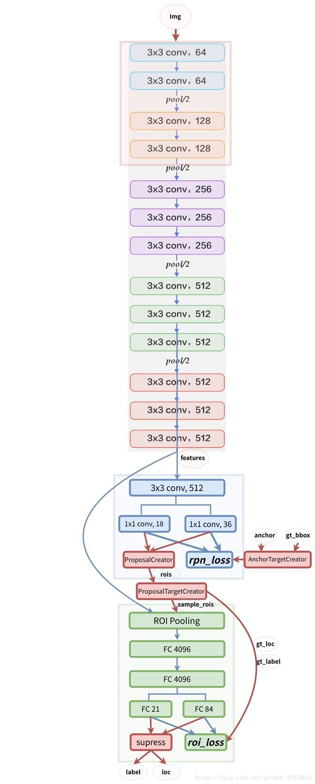Faster RCNN整体流程图，其中蓝线表示会进行反向传播，红线则不会

 

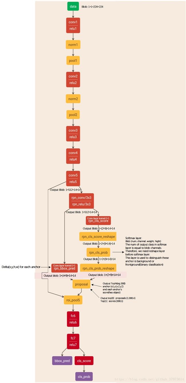有数据流的网络结构图《 参考》