Assignment | 02-week1 -Improving Deep Neural Networks_ Initialization_Part_1

该系列仅在原课程基础上课后作业部分添加个人学习笔记,如有错误，还请批评指教。在学习了 Andrew Ng 课程的基础上，为了更方便的查阅复习，将其整理成文字。因本人一直在学习英语，所以该系列以英文为主，同时也建议读者以英文为主，中文辅助，以便后期进阶时，为学习相关领域的学术论文做铺垫。- ZJ

Coursera 课程 |deeplearning.ai |网易云课堂

---

转载请注明作者和出处：ZJ 微信公众号-「SelfImprovementLab」

知乎：https://zhuanlan.zhihu.com/c_147249273

CSDN：http://blog.csdn.net/junjun_zhao/article/details/79087699

---

Welcome to the first assignment of “Improving Deep Neural Networks”.

Training your neural network requires specifying an initial value of the weights. A well chosen initialization method will help learning.

If you completed the previous course of this specialization, you probably followed our instructions for weight initialization, and it has worked out so far. But how do you choose the initialization for a new neural network? In this notebook, you will see how different initializations lead to different results. 不同的初始化会导致不同的结果。

A well chosen initialization can:
- Speed up the convergence of gradient descent 加快梯度下降的收敛
- Increase the odds of gradient descent converging to a lower training (and generalization) error 以较大几率使得梯度下降收敛到较低的训练(和泛化)误差。

To get started, run the following cell to load the packages and the planar dataset you will try to classify.

import numpy as np
import matplotlib.pyplot as plt
import sklearn
import sklearn.datasets
import scipy
from PIL import Image
from scipy import ndimage
from init_utils import sigmoid, relu, compute_loss, forward_propagation, backward_propagation
from init_utils import update_parameters, predict, load_dataset, plot_decision_boundary, predict_dec

%matplotlib inline
plt.rcParams['figure.figsize'] = (7.0, 4.0) # set default size of plots
plt.rcParams['image.interpolation'] = 'nearest'
plt.rcParams['image.cmap'] = 'gray'

# load image dataset: blue/red dots in circles
train_X, train_Y, test_X, test_Y = load_dataset()

def sigmoid(x):
    """
    Compute the sigmoid of x

    Arguments:
    x -- A scalar or numpy array of any size.

    Return:
    s -- sigmoid(x)
    """
    s = 1/(1+np.exp(-x))
    return s


def relu(x):
    """
    Compute the relu of x

    Arguments:
    x -- A scalar or numpy array of any size.

    Return:
    s -- relu(x)
    """
    s = np.maximum(0,x)

    return s


def compute_loss(a3, Y):

    """
    Implement the loss function

    Arguments:
    a3 -- post-activation, output of forward propagation
    Y -- "true" labels vector, same shape as a3

    Returns:
    loss - value of the loss function
    """

    m = Y.shape[1]
    logprobs = np.multiply(-np.log(a3),Y) + np.multiply(-np.log(1 - a3), 1 - Y)
    loss = 1./m * np.nansum(logprobs)

    return loss

def forward_propagation(X, parameters):
    """
    Implements the forward propagation (and computes the loss) presented in Figure 2.

    Arguments:
    X -- input dataset, of shape (input size, number of examples)
    Y -- true "label" vector (containing 0 if cat, 1 if non-cat)
    parameters -- python dictionary containing your parameters "W1", "b1", "W2", "b2", "W3", "b3":
                    W1 -- weight matrix of shape ()
                    b1 -- bias vector of shape ()
                    W2 -- weight matrix of shape ()
                    b2 -- bias vector of shape ()
                    W3 -- weight matrix of shape ()
                    b3 -- bias vector of shape ()

    Returns:
    loss -- the loss function (vanilla logistic loss)
    """

    # retrieve parameters
    W1 = parameters["W1"]
    b1 = parameters["b1"]
    W2 = parameters["W2"]
    b2 = parameters["b2"]
    W3 = parameters["W3"]
    b3 = parameters["b3"]

    # LINEAR -> RELU -> LINEAR -> RELU -> LINEAR -> SIGMOID
    z1 = np.dot(W1, X) + b1
    a1 = relu(z1)
    z2 = np.dot(W2, a1) + b2
    a2 = relu(z2)
    z3 = np.dot(W3, a2) + b3
    a3 = sigmoid(z3)

    cache = (z1, a1, W1, b1, z2, a2, W2, b2, z3, a3, W3, b3)

    return a3, cache


def backward_propagation(X, Y, cache):
    """
    Implement the backward propagation presented in figure 2.

    Arguments:
    X -- input dataset, of shape (input size, number of examples)
    Y -- true "label" vector (containing 0 if cat, 1 if non-cat)
    cache -- cache output from forward_propagation()

    Returns:
    gradients -- A dictionary with the gradients with respect to each parameter, activation and pre-activation variables
    """
    m = X.shape[1]
    (z1, a1, W1, b1, z2, a2, W2, b2, z3, a3, W3, b3) = cache

    dz3 = 1./m * (a3 - Y)
    dW3 = np.dot(dz3, a2.T)
    db3 = np.sum(dz3, axis=1, keepdims = True)

    da2 = np.dot(W3.T, dz3)
    dz2 = np.multiply(da2, np.int64(a2 > 0))
    dW2 = np.dot(dz2, a1.T)
    db2 = np.sum(dz2, axis=1, keepdims = True)

    da1 = np.dot(W2.T, dz2)
    dz1 = np.multiply(da1, np.int64(a1 > 0))
    dW1 = np.dot(dz1, X.T)
    db1 = np.sum(dz1, axis=1, keepdims = True)

    gradients = {"dz3": dz3, "dW3": dW3, "db3": db3,
                 "da2": da2, "dz2": dz2, "dW2": dW2, "db2": db2,
                 "da1": da1, "dz1": dz1, "dW1": dW1, "db1": db1}

    return gradients


def update_parameters(parameters, grads, learning_rate):
    """
    Update parameters using gradient descent

    Arguments:
    parameters -- python dictionary containing your parameters 
    grads -- python dictionary containing your gradients, output of n_model_backward

    Returns:
    parameters -- python dictionary containing your updated parameters 
                  parameters['W' + str(i)] = ... 
                  parameters['b' + str(i)] = ...
    """

    L = len(parameters) // 2 # number of layers in the neural networks

    # Update rule for each parameter
    for k in range(L):
        parameters["W" + str(k+1)] = parameters["W" + str(k+1)] - learning_rate * grads["dW" + str(k+1)]
        parameters["b" + str(k+1)] = parameters["b" + str(k+1)] - learning_rate * grads["db" + str(k+1)]

    return parameters


def predict(X, y, parameters):
    """
    This function is used to predict the results of a  n-layer neural network.

    Arguments:
    X -- data set of examples you would like to label
    parameters -- parameters of the trained model

    Returns:
    p -- predictions for the given dataset X
    """

    m = X.shape[1]
    p = np.zeros((1,m), dtype = np.int)

    # Forward propagation
    a3, caches = forward_propagation(X, parameters)

    # convert probas to 0/1 predictions
    for i in range(0, a3.shape[1]):
        if a3[0,i] > 0.5:
            p[0,i] = 1
        else:
            p[0,i] = 0

    # print results
    print("Accuracy: "  + str(np.mean((p[0,:] == y[0,:]))))

    return p


def load_dataset():
    np.random.seed(1)
    train_X, train_Y = sklearn.datasets.make_circles(n_samples=300, noise=.05)
    np.random.seed(2)
    test_X, test_Y = sklearn.datasets.make_circles(n_samples=100, noise=.05)
    # Visualize the data
    plt.scatter(train_X[:, 0], train_X[:, 1], c=train_Y, s=40, cmap=plt.cm.Spectral);
    train_X = train_X.T
    train_Y = train_Y.reshape((1, train_Y.shape[0]))
    test_X = test_X.T
    test_Y = test_Y.reshape((1, test_Y.shape[0]))
    return train_X, train_Y, test_X, test_Y


def plot_decision_boundary(model, X, y):
    # Set min and max values and give it some padding
    x_min, x_max = X[0, :].min() - 1, X[0, :].max() + 1
    y_min, y_max = X[1, :].min() - 1, X[1, :].max() + 1
    h = 0.01
    # Generate a grid of points with distance h between them
    xx, yy = np.meshgrid(np.arange(x_min, x_max, h), np.arange(y_min, y_max, h))
    # Predict the function value for the whole grid
    Z = model(np.c_[xx.ravel(), yy.ravel()])
    Z = Z.reshape(xx.shape)
    # Plot the contour and training examples
    plt.contourf(xx, yy, Z, cmap=plt.cm.Spectral)
    plt.ylabel('x2')
    plt.xlabel('x1')
    plt.scatter(X[0, :], X[1, :], c=np.squeeze(y), cmap=plt.cm.Spectral)
    plt.show()


def predict_dec(parameters, X):
    """
    Used for plotting decision boundary.

    Arguments:
    parameters -- python dictionary containing your parameters 
    X -- input data of size (m, K)

    Returns
    predictions -- vector of predictions of our model (red: 0 / blue: 1)
    """

    # Predict using forward propagation and a classification threshold of 0.5
    a3, cache = forward_propagation(X, parameters)
    predictions = (a3>0.5)
    return predictions

You would like a classifier to separate the blue dots from the red dots.

1 - Neural Network model

You will use a 3-layer neural network (already implemented for you). Here are the initialization methods you will experiment with:
- Zeros initialization – setting initialization = "zeros" in the input argument. 全 0 初始化
- Random initialization – setting initialization = "random" in the input argument. This initializes the weights to large random values. 随机初始化
- He initialization – setting initialization = "he" in the input argument. This initializes the weights to random values scaled according to a paper by He et al., 2015. He初始化方式（ paper by He et al., 2015. ）

Instructions: Please quickly read over the code below, and run it. In the next part you will implement the three initialization methods that this model() calls.

def model(X, Y, learning_rate = 0.01, num_iterations = 15000, print_cost = True, initialization = "he"):
    """
    Implements a three-layer neural network: LINEAR->RELU->LINEAR->RELU->LINEAR->SIGMOID. 三层神经网络

    Arguments:
    X -- input data, of shape (2, number of examples)
    Y -- true "label" vector (containing 0 for red dots; 1 for blue dots), of shape (1, number of examples)
    learning_rate -- learning rate for gradient descent 
    num_iterations -- number of iterations to run gradient descent
    print_cost -- if True, print the cost every 1000 iterations
    initialization -- flag to choose which initialization to use ("zeros","random" or "he")

    Returns:
    parameters -- parameters learnt by the model
    """

    grads = {}
    costs = [] # to keep track of the loss
    m = X.shape[1] # number of examples 样本数量 
    layers_dims = [X.shape[0], 10, 5, 1] # X.shape[0] 0 层 也就是 X 的特征 n_x ,接下来 1 2,3 层分别是 10 ，5 和 1 个 units

    # Initialize parameters dictionary.
    if initialization == "zeros":
        parameters = initialize_parameters_zeros(layers_dims)
    elif initialization == "random":
        parameters = initialize_parameters_random(layers_dims)
    elif initialization == "he":
        parameters = initialize_parameters_he(layers_dims)

    # Loop (gradient descent)

    for i in range(0, num_iterations):

        # Forward propagation: LINEAR -> RELU -> LINEAR -> RELU -> LINEAR -> SIGMOID.
        a3, cache = forward_propagation(X, parameters)

        # Loss
        cost = compute_loss(a3, Y)

        # Backward propagation.
        grads = backward_propagation(X, Y, cache)

        # Update parameters.
        parameters = update_parameters(parameters, grads, learning_rate)

        # Print the loss every 1000 iterations
        if print_cost and i % 1000 == 0:
            print("Cost after iteration {}: {}".format(i, cost))
            costs.append(cost)

    # plot the loss
    plt.plot(costs)
    plt.ylabel('cost')
    plt.xlabel('iterations (per hundreds)')
    plt.title("Learning rate =" + str(learning_rate))
    plt.show()

    return parameters

2 - Zero initialization

There are two types of parameters to initialize in a neural network: 两种类型的参数需要初始化
- the weight matrices (W[1],W[2],W[3],...,W[L−1],W[L]) ( W [ 1 ] , W [ 2 ] , W [ 3 ] , . . . , W [ L − 1 ] , W [ L ] ) 权重矩阵
- the bias vectors (b[1],b[2],b[3],...,b[L−1],b[L]) ( b [ 1 ] , b [ 2 ] , b [ 3 ] , . . . , b [ L − 1 ] , b [ L ] ) 偏差向量

Exercise: Implement the following function to initialize all parameters to zeros. You’ll see later that this does not work well since it fails to “break symmetry”, but lets try it anyway and see what happens. Use np.zeros((..,..)) with the correct shapes. 当所有参数初始化为 0 会发现 效果不好

# GRADED FUNCTION: initialize_parameters_zeros 

def initialize_parameters_zeros(layers_dims):
    """
    Arguments:
    layer_dims -- python array (list) containing the size of each layer.

    Returns:
    parameters -- python dictionary containing your parameters "W1", "b1", ..., "WL", "bL":
                    W1 -- weight matrix of shape (layers_dims[1], layers_dims[0])
                    b1 -- bias vector of shape (layers_dims[1], 1)
                    ...
                    WL -- weight matrix of shape (layers_dims[L], layers_dims[L-1])
                    bL -- bias vector of shape (layers_dims[L], 1)
    """

    parameters = {}
    L = len(layers_dims)            # number of layers in the network

    for l in range(1, L):
        ### START CODE HERE ### (≈ 2 lines of code)
        parameters['W' + str(l)] = np.zeros((layers_dims[l],layers_dims[l-1])) #回忆 w (n^[l],n^[l-1])
        parameters['b' + str(l)] = np.zeros((layers_dims[l],1)) #回忆 b (n^[l],1)
        ### END CODE HERE ###
    return parameters

# 错误：

# 参数拼错：layers_dims

# l 和 1 分清楚

parameters = initialize_parameters_zeros([3,2,1])
print("W1 = " + str(parameters["W1"]))
print("b1 = " + str(parameters["b1"]))
print("W2 = " + str(parameters["W2"]))
print("b2 = " + str(parameters["b2"]))

W1 = [[0. 0. 0.]
 [0. 0. 0.]]
b1 = [[0.]
 [0.]]
W2 = [[0. 0.]]
b2 = [[0.]]

Expected Output:

**W1**	[[ 0. 0. 0.] [ 0. 0. 0.]]
**b1**	[[ 0.] [ 0.]]
**W2**	[[ 0. 0.]]
**b2**	[[ 0.]]

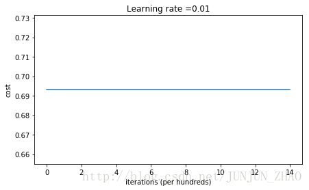
Run the following code to train your model on 15,000 iterations using zeros initialization.

parameters = model(train_X, train_Y, initialization = "zeros")
print ("On the train set:")
predictions_train = predict(train_X, train_Y, parameters)
print ("On the test set:")
predictions_test = predict(test_X, test_Y, parameters)

Cost after iteration 0: 0.6931471805599453
Cost after iteration 1000: 0.6931471805599453
Cost after iteration 2000: 0.6931471805599453
Cost after iteration 3000: 0.6931471805599453
Cost after iteration 4000: 0.6931471805599453
Cost after iteration 5000: 0.6931471805599453
Cost after iteration 6000: 0.6931471805599453
Cost after iteration 7000: 0.6931471805599453
Cost after iteration 8000: 0.6931471805599453
Cost after iteration 9000: 0.6931471805599453
Cost after iteration 10000: 0.6931471805599455
Cost after iteration 11000: 0.6931471805599453
Cost after iteration 12000: 0.6931471805599453
Cost after iteration 13000: 0.6931471805599453
Cost after iteration 14000: 0.6931471805599453

On the train set:
Accuracy: 0.5
On the test set:
Accuracy: 0.5

The performance is really bad, and the cost does not really decrease, and the algorithm performs no better than random guessing. Why? Lets look at the details of the predictions and the decision boundary:表现很差，损失没有下降 算法的表现 很差，对 训练集和 测试集的预测都是 0

print ("predictions_train = " + str(predictions_train))
print ("predictions_test = " + str(predictions_test))

predictions_train = [[0 0 0 0 0 0 0 0 0 0 0 0 0 0 0 0 0 0 0 0 0 0 0 0 0 0 0 0 0 0 0 0 0 0 0 0
  0 0 0 0 0 0 0 0 0 0 0 0 0 0 0 0 0 0 0 0 0 0 0 0 0 0 0 0 0 0 0 0 0 0 0 0
  0 0 0 0 0 0 0 0 0 0 0 0 0 0 0 0 0 0 0 0 0 0 0 0 0 0 0 0 0 0 0 0 0 0 0 0
  0 0 0 0 0 0 0 0 0 0 0 0 0 0 0 0 0 0 0 0 0 0 0 0 0 0 0 0 0 0 0 0 0 0 0 0
  0 0 0 0 0 0 0 0 0 0 0 0 0 0 0 0 0 0 0 0 0 0 0 0 0 0 0 0 0 0 0 0 0 0 0 0
  0 0 0 0 0 0 0 0 0 0 0 0 0 0 0 0 0 0 0 0 0 0 0 0 0 0 0 0 0 0 0 0 0 0 0 0
  0 0 0 0 0 0 0 0 0 0 0 0 0 0 0 0 0 0 0 0 0 0 0 0 0 0 0 0 0 0 0 0 0 0 0 0
  0 0 0 0 0 0 0 0 0 0 0 0 0 0 0 0 0 0 0 0 0 0 0 0 0 0 0 0 0 0 0 0 0 0 0 0
  0 0 0 0 0 0 0 0 0 0 0 0]]
predictions_test = [[0 0 0 0 0 0 0 0 0 0 0 0 0 0 0 0 0 0 0 0 0 0 0 0 0 0 0 0 0 0 0 0 0 0 0 0
  0 0 0 0 0 0 0 0 0 0 0 0 0 0 0 0 0 0 0 0 0 0 0 0 0 0 0 0 0 0 0 0 0 0 0 0
  0 0 0 0 0 0 0 0 0 0 0 0 0 0 0 0 0 0 0 0 0 0 0 0 0 0 0 0]]

plt.title("Model with Zeros initialization")
axes = plt.gca()
axes.set_xlim([-1.5,1.5])
axes.set_ylim([-1.5,1.5])
plot_decision_boundary(lambda x: predict_dec(parameters, x.T), train_X, train_Y)
# 这里一直出错，因为是本地跑程序，不是在coursera 上 所以在
# def plot_decision_boundary(model, X, y):
#     plt.scatter(X[0, :], X[1, :], c=np.squeeze(y), cmap=plt.cm.Spectral)
#  c=np.squeeze(y) 要对 y 进行 np.squeeze

The model is predicting 0 for every example.

In general, initializing all the weights to zero results in the network failing to break symmetry. This means that every neuron in each layer will learn the same thing, and you might as well be training a neural network with n[l]=1 n [ l ] = 1 for every layer, and the network is no more powerful than a linear classifier such as logistic regression.

What you should remember:
- The weights W[l] W [ l ] should be initialized randomly to break symmetry. 采用随机初始化 打破对称性
- It is however okay to initialize the biases b[l] b [ l ] to zeros. Symmetry is still broken so long as W[l] W [ l ] is initialized randomly. 对于参数 b 是可以初始化为 0 的

3 - Random initialization

To break symmetry, lets intialize the weights randomly. Following random initialization, each neuron can then proceed to learn a different function of its inputs. In this exercise, you will see what happens if the weights are intialized randomly, but to very large values.

Exercise: Implement the following function to initialize your weights to large random values (scaled by *10) and your biases to zeros. Use np.random.randn(..,..) * 10 for weights and np.zeros((.., ..)) for biases. We are using a fixed np.random.seed(..) to make sure your “random” weights match ours, so don’t worry if running several times your code gives you always the same initial values for the parameters.

# GRADED FUNCTION: initialize_parameters_random

def initialize_parameters_random(layers_dims):
    """
    Arguments:
    layer_dims -- python array (list) containing the size of each layer.

    Returns:
    parameters -- python dictionary containing your parameters "W1", "b1", ..., "WL", "bL":
                    W1 -- weight matrix of shape (layers_dims[1], layers_dims[0])
                    b1 -- bias vector of shape (layers_dims[1], 1)
                    ...
                    WL -- weight matrix of shape (layers_dims[L], layers_dims[L-1])
                    bL -- bias vector of shape (layers_dims[L], 1)
    """

    np.random.seed(3)               # This seed makes sure your "random" numbers will be the as ours
    parameters = {}
    L = len(layers_dims)            # integer representing the number of layers

    for l in range(1, L):
        ### START CODE HERE ### (≈ 2 lines of code)
        parameters['W' + str(l)] = np.random.randn(layers_dims[l],layers_dims[l-1])*10
        parameters['b' + str(l)] = np.zeros((layers_dims[l],1))
        ### END CODE HERE ###

    return parameters

parameters = initialize_parameters_random([3, 2, 1])
print("W1 = " + str(parameters["W1"]))
print("b1 = " + str(parameters["b1"]))
print("W2 = " + str(parameters["W2"]))
print("b2 = " + str(parameters["b2"]))

W1 = [[ 17.88628473   4.36509851   0.96497468]
 [-18.63492703  -2.77388203  -3.54758979]]
b1 = [[0.]
 [0.]]
W2 = [[-0.82741481 -6.27000677]]
b2 = [[0.]]

Expected Output:

**W1**	[[ 17.88628473 4.36509851 0.96497468] [-18.63492703 -2.77388203 -3.54758979]]
**b1**	[[ 0.] [ 0.]]
**W2**	[[-0.82741481 -6.27000677]]
**b2**	[[ 0.]]

Run the following code to train your model on 15,000 iterations using random initialization.

parameters = model(train_X, train_Y, initialization = "random")
print ("On the train set:")
predictions_train = predict(train_X, train_Y, parameters)
print ("On the test set:")
predictions_test = predict(test_X, test_Y, parameters)

d:\program files\python36\lib\site-packages\ipykernel_launcher.py:44: RuntimeWarning: divide by zero encountered in log
d:\program files\python36\lib\site-packages\ipykernel_launcher.py:44: RuntimeWarning: invalid value encountered in multiply


Cost after iteration 0: inf
Cost after iteration 1000: 0.6243339944795463
Cost after iteration 2000: 0.5983698376976234
Cost after iteration 3000: 0.5640713641303857
Cost after iteration 4000: 0.5502225777263651
Cost after iteration 5000: 0.5445189912897229
Cost after iteration 6000: 0.5374939942050982
Cost after iteration 7000: 0.47927872911735586
Cost after iteration 8000: 0.39787508336662053
Cost after iteration 9000: 0.3934925383461005
Cost after iteration 10000: 0.3920373161708829
Cost after iteration 11000: 0.38930570830972355
Cost after iteration 12000: 0.3861562072516527
Cost after iteration 13000: 0.38499595295812233
Cost after iteration 14000: 0.38280923039736164

On the train set:
Accuracy: 0.83
On the test set:
Accuracy: 0.86

If you see “inf” as the cost after the iteration 0, this is because of numerical roundoff; a more numerically sophisticated implementation would fix this. But this isn’t worth worrying about for our purposes.

Anyway, it looks like you have broken symmetry, and this gives better results. than before. The model is no longer outputting all 0s.

print (predictions_train)
print (predictions_test)

[[1 0 1 1 0 0 1 1 1 1 1 0 1 0 0 1 0 1 1 0 0 0 1 0 1 1 1 1 1 1 0 1 1 0 0 1
  1 1 1 1 1 1 1 0 1 1 1 1 0 1 0 1 1 1 1 0 0 1 1 1 1 0 1 1 0 1 0 1 1 1 1 0
  0 0 0 0 1 0 1 0 1 1 1 0 0 1 1 1 1 1 1 0 0 1 1 1 0 1 1 0 1 0 1 1 0 1 1 0
  1 0 1 1 0 0 1 0 0 1 1 0 1 1 1 0 1 0 0 1 0 1 1 1 1 1 1 1 0 1 1 0 0 1 1 0
  0 0 1 0 1 0 1 0 1 1 1 0 0 1 1 1 1 0 1 1 0 1 0 1 1 0 1 0 1 1 1 1 0 1 1 1
  1 0 1 0 1 0 1 1 1 1 0 1 1 0 1 1 0 1 1 0 1 0 1 1 1 0 1 1 1 0 1 0 1 0 0 1
  0 1 1 0 1 1 0 1 1 0 1 1 1 0 1 1 1 1 0 1 0 0 1 1 0 1 1 1 0 0 0 1 1 0 1 1
  1 1 0 1 1 0 1 1 1 0 0 1 0 0 0 1 0 0 0 1 1 1 1 0 0 0 0 1 1 1 1 0 0 1 1 1
  1 1 1 1 0 0 0 1 1 1 1 0]]
[[1 1 1 1 0 1 0 1 1 0 1 1 1 0 0 0 0 1 0 1 0 0 1 0 1 0 1 1 1 1 1 0 0 0 0 1
  0 1 1 0 0 1 1 1 1 1 0 1 1 1 0 1 0 1 1 0 1 0 1 0 1 1 1 1 1 1 1 1 1 0 1 0
  1 1 1 1 1 0 1 0 0 1 0 0 0 1 1 0 1 1 0 0 0 1 1 0 1 1 0 0]]

plt.title("Model with large random initialization")
axes = plt.gca()
axes.set_xlim([-1.5,1.5])
axes.set_ylim([-1.5,1.5])
plot_decision_boundary(lambda x: predict_dec(parameters, x.T), train_X, train_Y)

Observations:
- The cost starts very high. This is because with large random-valued weights, the last activation (sigmoid) outputs results that are very close to 0 or 1 for some examples, and when it gets that example wrong it incurs a very high loss for that example. Indeed, when log(a[3])=log(0) log ⁡ ( a [ 3 ] ) = log ⁡ ( 0 ) , the loss goes to infinity.
- Poor initialization can lead to vanishing/exploding gradients, which also slows down the optimization algorithm. 糟糕的 初始化 会导致梯度爆炸或消失
- If you train this network longer you will see better results, but initializing with overly large random numbers slows down the optimization.

In summary:
- Initializing weights to very large random values does not work well.
- Hopefully intializing with small random values does better. The important question is: how small should be these random values be? Lets find out in the next part!

4 - He initialization

Finally, try “He Initialization”; this is named for the first author of He et al., 2015. (If you have heard of “Xavier initialization”, this is similar except Xavier initialization uses a scaling factor for the weights W[l] W [ l ] of sqrt(1./layers_dims[l-1]) where He initialization would use sqrt(2./layers_dims[l-1]).)

Exercise: Implement the following function to initialize your parameters with He initialization.

Hint: This function is similar to the previous initialize_parameters_random(...). The only difference is that instead of multiplying np.random.randn(..,..) by 10, you will multiply it by 2dimension of the previous layer‾‾‾‾‾‾‾‾‾‾‾‾‾‾‾‾‾‾‾‾‾√ 2 dimension of the previous layer , which is what He initialization recommends for layers with a ReLU activation.

He初始化方式（He et al., 2015.）正是为解决上面问题而提出的。这种初始化方式是对随机初始化的权重矩阵乘以sqrt(2./layers_dims[l-1]))。另一种相识的初始化方式Xavier 方式，也顺便提下，是对权重矩阵乘以sqrt(1./layers_dims[l-1])。

# GRADED FUNCTION: initialize_parameters_he

def initialize_parameters_he(layers_dims):
    """
    Arguments:
    layer_dims -- python array (list) containing the size of each layer.

    Returns:
    parameters -- python dictionary containing your parameters "W1", "b1", ..., "WL", "bL":
                    W1 -- weight matrix of shape (layers_dims[1], layers_dims[0])
                    b1 -- bias vector of shape (layers_dims[1], 1)
                    ...
                    WL -- weight matrix of shape (layers_dims[L], layers_dims[L-1])
                    bL -- bias vector of shape (layers_dims[L], 1)
    """

    np.random.seed(3)
    parameters = {}
    L = len(layers_dims) - 1 # integer representing the number of layers

    for l in range(1, L + 1):
        ### START CODE HERE ### (≈ 2 lines of code)
        parameters['W' + str(l)] = np.random.randn(layers_dims[l],layers_dims[l-1])*np.sqrt(2./layers_dims[l-1])
        parameters['b' + str(l)] = np.zeros((layers_dims[l],1))
        ### END CODE HERE ###

    return parameters

parameters = initialize_parameters_he([2, 4, 1])
print("W1 = " + str(parameters["W1"]))
print("b1 = " + str(parameters["b1"]))
print("W2 = " + str(parameters["W2"]))
print("b2 = " + str(parameters["b2"]))

W1 = [[ 1.78862847  0.43650985]
 [ 0.09649747 -1.8634927 ]
 [-0.2773882  -0.35475898]
 [-0.08274148 -0.62700068]]
b1 = [[0.]
 [0.]
 [0.]
 [0.]]
W2 = [[-0.03098412 -0.33744411 -0.92904268  0.62552248]]
b2 = [[0.]]

Expected Output:

**W1**	[[ 1.78862847 0.43650985] [ 0.09649747 -1.8634927 ] [-0.2773882 -0.35475898] [-0.08274148 -0.62700068]]
**b1**	[[ 0.] [ 0.] [ 0.] [ 0.]]
**W2**	[[-0.03098412 -0.33744411 -0.92904268 0.62552248]]
**b2**	[[ 0.]]

Run the following code to train your model on 15,000 iterations using He initialization.

parameters = model(train_X, train_Y, initialization = "he")
print ("On the train set:")
predictions_train = predict(train_X, train_Y, parameters)
print ("On the test set:")
predictions_test = predict(test_X, test_Y, parameters)

Cost after iteration 0: 0.8830537463419761
Cost after iteration 1000: 0.6879825919728063
Cost after iteration 2000: 0.6751286264523371
Cost after iteration 3000: 0.6526117768893807
Cost after iteration 4000: 0.6082958970572938
Cost after iteration 5000: 0.5304944491717495
Cost after iteration 6000: 0.4138645817071795
Cost after iteration 7000: 0.31178034648444414
Cost after iteration 8000: 0.23696215330322562
Cost after iteration 9000: 0.18597287209206836
Cost after iteration 10000: 0.15015556280371808
Cost after iteration 11000: 0.12325079292273551
Cost after iteration 12000: 0.09917746546525934
Cost after iteration 13000: 0.08457055954024277
Cost after iteration 14000: 0.07357895962677363

On the train set:
Accuracy: 0.9933333333333333
On the test set:
Accuracy: 0.96

plt.title("Model with He initialization")
axes = plt.gca()
axes.set_xlim([-1.5,1.5])
axes.set_ylim([-1.5,1.5])
plot_decision_boundary(lambda x: predict_dec(parameters, x.T), train_X, train_Y)

Observations:
- The model with He initialization separates the blue and the red dots very well in a small number of iterations.

5 - Conclusions

You have seen three different types of initializations. For the same number of iterations and same hyperparameters the comparison is:

**Model**	**Train accuracy**	**Problem/Comment**
3-layer NN with zeros initialization	50%	fails to break symmetry
3-layer NN with large random initialization	83%	too large weights
3-layer NN with He initialization	99%	recommended method

What you should remember from this notebook:
- Different initializations lead to different results
- Random initialization is used to break symmetry and make sure different hidden units can learn different things
- Don’t intialize to values that are too large
- He initialization works well for networks with ReLU activations.

---

PS: 欢迎扫码关注公众号：「SelfImprovementLab」！专注「深度学习」，「机器学习」，「人工智能」。以及 「早起」，「阅读」，「运动」，「英语 」「其他」不定期建群 打卡互助活动。