Coursera | Andrew Ng (02-week-2-2.2)—理解 mini-batch 梯度下降法
该系列仅在原课程基础上部分知识点添加个人学习笔记,或相关推导补充等。如有错误,还请批评指教。在学习了 Andrew Ng 课程的基础上,为了更方便的查阅复习,将其整理成文字。因本人一直在学习英语,所以该系列以英文为主,同时也建议读者以英文为主,中文辅助,以便后期进阶时,为学习相关领域的学术论文做铺垫。- ZJ
Coursera 课程 |deeplearning.ai |网易云课堂
转载请注明作者和出处:ZJ 微信公众号-「SelfImprovementLab」
知乎:https://zhuanlan.zhihu.com/c_147249273
CSDN:http://blog.csdn.net/JUNJUN_ZHAO/article/details/79098516
2.2 Understanding Mini-batch Gradient descent (理解 mini-batch 梯度下降法 )
(字幕来源:网易云课堂)
In the previous video, you saw how you can use mini-batch gradient descent to start making progress and start taking gradient descent steps,even when you’re just partway through processing your training set,even for the first time.In this video, you learn more details of how to implement gradient descent and gain a better understanding of what it’s doing and why it works.
在上周视频中你知道了如何利用 mini-batch 梯度下降法,来开始处理训练集和开始梯度下降,即使你只处理了部分训练集,即使你是第一次处理,本视频中,我们将进一步学习如何执行梯度下降法,更好地理解其作用和原理。
With batch gradient descent on every iteration you go through the entire training set and you’d expect the cost to go down on every single iteration.So if we’ve had the cost function J as a function of different iterations,it should decrease on every single iteration.And if it ever goes up even on one iteration then something is wrong.Maybe you’re running ways too big.On mini batch gradient descent though,if you plot progress on your cost function,then it may not decrease on every iteration.In particular, on every iteration you’re processing some X{t} , Y{t} ,and so if you plot the cost function J{t} ,which is computer using just X{t} , Y{t} .Then it’s as if on every iteration you’re training on a different training set or really training on a different mini batch.So you plot the cost function J,you’re more likely to see something that looks like this.It should trend downwards, but it’s also going to be a little bit noisier.So if you plot J{t} ,as you’re training mini batch in descent it may be over multiple epochs,you might expect to see a curve like this.So it’s okay if it doesn’t go down on every iteration.But it should trend downwards,and the reason it’ll be a little bit noisy is that,maybe X{1} , Y{1} is just the rows of easy mini batch,so your cost might be a bit lower,but then maybe just by chance, X{2} , Y{2} is just a harder mini batch.Maybe you needed some mislabeled examples in it,in which case the cost will be a bit higher and so on.So that’s why you get these oscillations,as you plot the cost when you’re running mini batch gradient descent.
使用 batch 梯度下降法时,每次迭代你都需要历遍整个训练集,可以预期每次迭代的成本都会下降,所以如果成本函数 J 是迭代次数的一个函数,它应该会随着每次迭代而减少,如果 J 在某次迭代中增加了 那肯定出了问题,也许你的运行方式太大,使用 mini-batch 梯度下降法,如果你作出成本函数在整个过程中的图,则并不是每次迭代都是下降的,特别是在每次迭代中,你要处理的是 X{t} Y{t} ,如果要作出成本函数 J{t} 的图,而 J{t} 只和 X{t} Y{t} 有关,也就是每次迭代下你都在训练不同的样本集,或者说训练不同的 mini-batch ,如果你要作出成本函数 J 的图,你很可能会看到这样的结果,走向朝下 但有更多的噪声,所以如果你作 J{t} 的图,因为在训练 mini-batch 梯度下降法时会经过多代,你可能会看到这样的曲线,没有每次迭代都下降是不要紧的,但是走势应该向下,噪声产生的原因在于也许 X{1} 和 Y{1} 是比较容易计算的 mini-batch ,因此成本会低一些,不过也许出于偶然, X{2} Y{2} 是比较难运算的 mini-batch ,或许你需要一些残缺的样本,这样一来成本会更高一些,所以才回出现这些摆动,因为你是在运行 mini-batch 梯度下降法作出成本函数图。
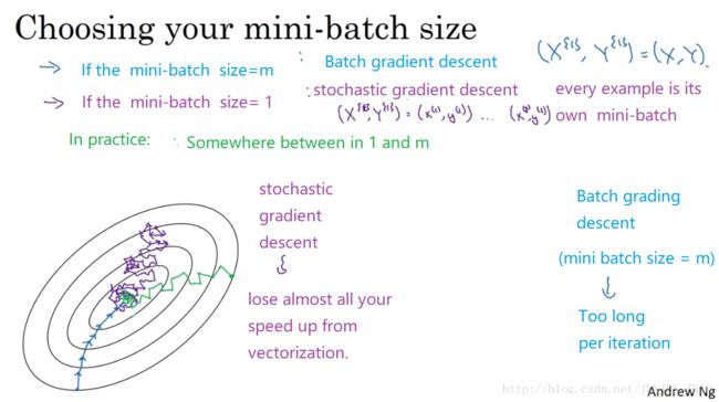
Now one of the parameters you need to choose is the size of your mini batch.So m was the training set size.On one extreme, if the mini-batch size=m then you just end up with batch gradient descent.Al right, so in this extreme you would just have one mini-batch X{1} , Y{1} ,and this mini-batch is equal to your entire training set.So setting a mini-batch size m just gives you batch gradient descent.The other extreme would be if your mini-batch size, were = 1.This gives you an algorithm called stochastic gradient descent.And here every example is its own mini-batch .So what you do in this case is you look at the first mini-batch ,so X{1} , Y{1} ,but when your mini-batch size is one,this just has your first training example,and you take derivative to sense that were your first training example.And then you next take a look at your second mini-batch ,which is just your second training example,and take your gradient descent step with that,and then you do it with the third training example and so on,looking at just one single training sample at the time.
你需要决定的变量之一是 mini-batch 的大小,m 就是训练集的大小,极端情况下 如果 mini-batch 的大小 = m,其实就是 batch 梯度下降法,在这种极端情况下 你就有了 mini-batch X{1} Y{1} ,并且该 mini-batch 等于整个训练集,所以把 mini-batch 大小设为 m 可以得到 batch梯度下降法,另一个极端情况 假设 mini-batch 大小为 1,就有了新的算法 叫做随机梯度下降法,每个样本都是独立的 mini-batch ,当你看第一个 mini-batch ,也就是 X{1} 和 Y{1} ,如果 mini-batch 大小为1,它就是你的第一个训练样本,这就是你的第一个训练样本,接着再看第二个 mini-batch ,也就是第二个训练样本,采取梯度下降步骤,然后是第三个训练样本 以此类推,一次只处理一个。
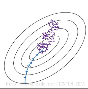
So let’s look at what these two extremes will do on optimizing this cost function.If these are the contours of the cost function you’re trying to minimize,so your minimum is there.Then batch gradient descent might start somewhere and be able to take relatively low noise, relatively large steps.And you just keep matching to the minimum.In contrast with stochastic gradient descent If you start somewhere let’s pick a different starting point.Then on every iteration,you’re taking gradient descent with just a single training example so most of the time you hit towards the global minimum.But sometimes you hit in the wrong direction,if that one example happens to point you in a bad direction.So stochastic gradient descent can be extremely noisy.And on average, it’ll take you in a good direction,but sometimes it’ll head in the wrong direction as well.As stochastic gradient descent won’t ever converge,it’ll always just kind of oscillate and wander around the region of the minimum,but it won’t ever just head to the minimum and stay there.

看在两个极端下 成本函数的优化情况,如果这是你想要最小化的成本函数的轮廓,最小值在那里,batch 梯度下降从某处开始,相对噪声低些,幅度也大一些,你可以继续找最小值,相反 在随机梯度下降法中,从某一点开始 我们重新选取一个起始点,每次迭代,你只对一个样本进行梯度下降,大部分时候你向着全局最小值靠近,有时候你会远离最小值,因为那个样本恰好给你指的方向不对,因此随机梯度下降法是有很多噪声的,平均来看 它最终会靠近最小值,不过有时候也会方向错误,因为随机梯度下降法永远不会收敛,而是会一直在最小值附近波动,但它并不会在达到最小值并停留在此。
In practice, the mini-batch size you use will be somewhere in between.Somewhere between in 1 and m,and 1 and m are respectively too small and too large.And here’s why.If you use batch grading descent,so this is your mini batch size equals m.Then you’re processing a huge training set on every iteration.So the main disadvantage of this is that it takes too much time too long per iteration,assuming you have a very long training set.If you have a small training set then batch gradient descent is fine.If you go to the opposite, if you use stochastic gradient descent,then it’s nice that you get to make progress after processing just 1 example.that’s actually not a problem.And the noisiness can be ameliorated 改善 or can be reduced by just using a smaller learning rate.But a huge disadvantage to stochastic gradient descent is that you lose almost all your speed up from vectorization.Because, here you’re processing a single training example at a time.The way you process each example is going to be very inefficient.
实际上你选择的 mini-batch 大小在二者之间,大小在 1 和 m 之间,而 1 太小了 m 太大了,原因在于,如果使用 batch 梯度下降法, mini-batch 的大小为 m,每个迭代需要处理大量训练样本,该算法的主要弊端在于特别是在训练样本数量巨大的时候,单次迭代耗时太长,如果训练样本不大 batch 梯度下降法运行地很好,相反 如果使用随机梯度下降法,如果你只要处理 1 个样本,那这个方法很好,这样做没有问题,通过减小学习率,噪声会被改善或有所减少,但随机梯度下降法的一大缺点是,你会失去所有向量化带给你的加速,因为一次性只处理了一个训练样本,这样效率过于低下。
So what works best in practice is something in between where you have some Mini-batch size not too big or too small.And this gives you in practice the fastest learning.And you notice that this has two good things going for it.One is that you do get a lot of vectorization.So in the example we used on the previous video,if your mini batch size was 1000 examples,then, you might be able to vectorize across 1000 examples which is going to be much faster than processing the examples one at a time.And second, you can also make progress,without needing to wait till you process the entire training set.So again using the numbers we have from the previous video,each epoch or each part your training set allows you to see 5,000 gradient descent steps.So in practice they’ll be some in-between mini-batch size that works best.And so with mini-batch gradient descent,we start here, maybe one iteration does this, two iterations, three, four.And It’s not guaranteed to always head toward the minimum,but it tends to head more consistently in direction of the minimum than the consequent descent.And then it doesn’t always exactly converge or oscillate in a very small region.If that’s an issue you can always reduce the learning rate slowly.We’ll talk more about learning rate decayor how to reduce the learning rate in a later video.
所以实践中最好选择不大不小的 Mini-batch 尺寸,实际上学习率达到最快,你会发现两个好处,一方面 你得到了大量向量化,上个视频中我们用过的例子中,如果 mini-batch 大小为 1000 个样本,你就可以对 1000 个样本向量化,你多次处理样本要快得多,另一方面 你不需要等待整个训练集被处理完,就可以开始进行后续工作,再用一下上个视频的数字,每代训练集允许我们采取 5000 个梯度下降步骤,所以实际上一些位于中间的 mini-batch 大小效果最好,用 mini-batch 梯度下降法,我们从这里开始 一次迭代这样做 两次 三次 四次,它不会总朝向最小值靠近,但它比随机梯度下降要更持续地靠近最小值的方向,它也不一定在很小的范围内收敛或者波动,如果出现这个问题 可以慢慢减少学习率,我们在下个视频会讲到学习率衰减,也就是如何减少学习率。
So if the mini-batch size should not be m and should not be 1,but should be something in between, how do you go about choosing it?Well, here are some guidelines.First, if you have a small training set,just use batch gradient descent.If you have a small training set then no point using mini-batch gradient descent you can process a whole training set quite fast.So you might as well use batch gradient descent.What a small training set means,I would say if it’s less than maybe 2000 it’d be perfectly fine to just use batch gradient descent.Otherwise, if you have a bigger training set,typical mini batch sizes would be, anything from 64 up to maybe 512 are quite typical.And because of the way computer memory is laid out and accessed,sometimes your code runs faster if your mini-batch size is a power of 2.All right, so 64 is 2 to the 6th,2 to the 7th, 2 to the 8, 2 to the 9,so often I’ll implement my mini-batch size to be a power of 2.I know that in a previous video I used a mini-batch size of 1000 ,if you really wanted to do that I would recommend you just use your 1024,which is 2 to the power of 10.And you do see mini batch sizes of size 1024, it is a bit more rare.This range of mini batch sizes, a little bit more common.One last tip is to make sure that your mini batch,All of your X{t} , Y{t} that fits in CPU/GPU memory.And this really depends on your application and how large a single training sample is.But if you ever process a mini-batch that doesn’t actually fit in CPU, GPU memory,whether you’re using the process, the data.Then you find that the performance suddenly falls of a cliffand is suddenly much worse.
如果 mini-batch 大小既不是 1 也不是 m,应该取中间值 那应该怎们选择呢,其实是有指导原则的,首先 如果训练集较小,直接使用 batch 梯度下降法,样本集较小就没必要使用 mini-batch 梯度下降法,你可以快速处理整个训练集,所以使用 batch 梯度下降法也很好,这里的少是说小于 2000 个样本,这样比较适合使用 batch 梯度下降法,不然 样本数目较大的话,一般的 mini-batch 大小为 64 到 512,考虑到电脑内存设置和使用的方式,如果 mini-batch 大小是 2 的次方,代码会运行地快一些, 64 就是 2 的 6 次方,以此类推 2 的 7 次方 8 次方 9 次方,所以我经常把 min-batch 大小设成 2 次方,在上个视频里 我的 mini-batch 大小设为了 1000 ,建议你可以试一下 1024,也就是 2 的 10 次方,也有 mini-batch 的大小为 1024 不过比较少见,这个区间大小的 mini-batch 比较常见,最后要注意的是 在你的 mini-batch 中, X{t} 和 Y{t} 要符合CPU/GPU内存,取决于你的应用方向,以及训练集的大小,如果你处理的 mini-batch 和 CPU/GPU 内存不相符,不管你用什么方法处理数据,你会注意到算法的表现急转直下,变得惨不忍睹,
So I hope this gives you a sense of the typical range of mini batch sizes that people use.In practice of course the mini batch size is another hyper parameterthat you might do a quick search over to try to figure out which one is most sufficient of reducing the cost function J.So what i would do is just try several different values.Try a few different powers of two and then see if you can pick one that makes your gradient descent optimization algorithm as efficient as possible.But hopefully this gives you a set of guidelines for how to get started with that hyper parameter search.You now know how to implement mini-batch gradient descent,and make your algorithm run much faster,especially when you’re training on a large training set.But it turns out there’re even more efficient algorithms than gradient descent or mini-batch gradient descent.Let’s start talking about them in the next few videos.
所以你要知道一般人们使用的 mini-batch 大小,事实上 mini-batch 大小是另一个重要的变量,你需要做一个快速尝试,才能找到能够最有效地减少成本函数的那个,我一般会尝试几个不同的值,几个不同的 2 次方 然后看能否找到一个,让梯度下降优化算法最高效的大小,希望这些能够指导你,如何开始找到这一数值,你学会了如何执行 mini-batch 梯度下降,令算法运行得更快, 特别是在训练样本数目较大的情况下,不过还有个更加高效的算法,比梯度下降法和 mini-batch 梯度下降法都要高效的多,我们在接下来的视频中将为大家一一讲解。
重点总结:
不同 size 大小的比较
普通的 batch 梯度下降法和 Mini-batch 梯度下降法代价函数的变化趋势,如下图所示:
batch梯度下降:
- 对所有 m 个训练样本执行一次梯度下降,每一次迭代时间较长;
- Cost function 总是向减小的方向下降。
随机梯度下降:
- 对每一个训练样本执行一次梯度下降,但是丢失了向量化带来的计算加速;
- Cost function 总体的趋势向最小值的方向下降,但是无法到达全局最小值点,呈现波动的形式。
Mini-batch梯度下降:
- 选择一个 1<size<m 的合适的size进行Mini-batch梯度下降,可以实现快速学习,也应用了向量化带来的好处。
- Cost function 的下降处于前两者之间。
Mini-batch 大小的选择
- 如果训练样本的大小比较小时,如 m⩽ 2000 时 —— 选择 batch 梯度下降法;
- 如果训练样本的大小比较大时,典型的大小为:
26、27、⋯、210 ; - Mini-batch 的大小要符合 CPU/GPU 内存。
参考文献:
[1]. 大树先生.吴恩达Coursera深度学习课程 DeepLearning.ai 提炼笔记(2-2)– 优化算法
PS: 欢迎扫码关注公众号:「SelfImprovementLab」!专注「深度学习」,「机器学习」,「人工智能」。以及 「早起」,「阅读」,「运动」,「英语 」「其他」不定期建群 打卡互助活动。


