吴恩达深度学习(一)-第三周：Planar data classification with one hidden layer

Planar data classification with one hidden layer

本练习会建立只有一个隐藏层的神经网络，我们将看到这与逻辑回归有多大的差别。

You will learn how to:

• 用一个隐藏层的神经网络实现二分类
• 在神经元上使用非线性激活函数, such as tanh
• 计算交叉熵代价函数
• 实现正向传播和反向传播

1 - Packages

Let’s first import all the packages that you will need during this assignment.

• numpy is the fundamental package for scientific computing with Python.
• sklearn provides simple and efficient tools for data mining and data analysis.
• matplotlib is a library for plotting graphs in Python.
• testCases provides some test examples to assess the correctness of your functions
• planar_utils provide various useful functions used in this assignment

# Package imports
import numpy as np
import matplotlib.pyplot as plt
from testCases import *
import sklearn
import sklearn.datasets
import sklearn.linear_model
from planar_utils import plot_decision_boundary, sigmoid, load_planar_dataset, load_extra_datasets

%matplotlib inline

np.random.seed(1) # set a seed so that the results are consistent

2 - Dataset

首先，让我们来获取数据集。

X, Y = load_planar_dataset()  # 作业提供的函数，感兴趣自信查看源码
X.shape, Y.shape
# ((2, 400), (1, 400))

# Visualize the data:
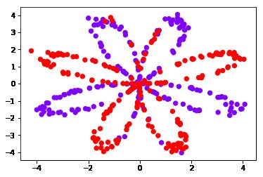
plt.scatter(X[0, :], X[1, :], c=Y.flatten(), s=40, cmap='rainbow');

You have:
- a numpy-array (matrix) X that contains your features (x1, x2)
- a numpy-array (vector) Y that contains your labels (red:0, blue:1).

### START CODE HERE ### (≈ 3 lines of code)
shape_X = X.shape
shape_Y = Y.shape
m = shape_X[1]  # training set size
### END CODE HERE ###

print ('The shape of X is: ' + str(shape_X))
print ('The shape of Y is: ' + str(shape_Y))
print ('I have m = %d training examples!' % (m))

The shape of X is: (2, 400)
The shape of Y is: (1, 400)
I have m = 400 training examples!

Expected Output:
​

**shape of X** (2, 400) **shape of Y** (1, 400)

**m**
 400  

3 - Simple Logistic Regression

在构造神经网络前，首先来看看逻辑回归在这个问题的表现。

# Train the logistic regression classifier
clf = sklearn.linear_model.LogisticRegressionCV();
# 传入逻辑回归中的话，X和Y 要把每条样本按行排列
clf.fit(X.T, Y.T);

D:\Anaconda3\envs\Tensorflow\lib\site-packages\sklearn\utils\validation.py:578: DataConversionWarning: A column-vector y was passed when a 1d array was expected. Please change the shape of y to (n_samples, ), for example using ravel().
  y = column_or_1d(y, warn=True)

# Plot the decision boundary for logistic regression
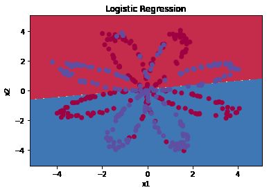
plot_decision_boundary(lambda x: clf.predict(x), X, Y)
plt.title("Logistic Regression")

# Print accuracy
LR_predictions = clf.predict(X.T)
# 前一项计算预测正样本正确的数量，后一项计算预测负样本正确的数量。
print ('Accuracy of logistic regression: %d ' % float((np.dot(Y,LR_predictions) + np.dot(1-Y,1-LR_predictions))/float(Y.size)*100) +
       '% ' + "(percentage of correctly labelled datapoints)")

Accuracy of logistic regression: 47 % (percentage of correctly labelled datapoints)

​

Expected Output:

**Accuracy**

47%

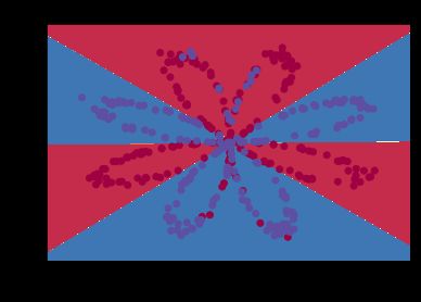
本数据集是非线性可分的，所有逻辑回归变现不好。接下来看看神经网络的表现。

4 - Neural Network model

Logistic regression did not work well on the “flower dataset”. You are going to train a Neural Network with a single hidden layer.

Here is our model:

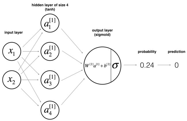
Mathematically:

For one example $x^{(i)}$:
$$z^{[1](i)}=W^{[1]}{x}^{(i)}+b^{[1](i)}\text{\hspace{1em}(1)}$$
$$a^{[1](i)}=\tanh (z^{[1](i)})\text{\hspace{1em}(2)}$$
$$z^{[2](i)}=W^{[2]}{a}^{[1](i)}+b^{[2](i)}\text{\hspace{1em}(3)}$$
$${\hat{y}}^{(i)}=a^{[2](i)}=\sigma (z^{[2](i)})\text{\hspace{1em}(4)}$$
KaTeX parse error: Expected & or \\ or \cr or \end at position 42: …gin{cases} 1 & \̲m̲b̲o̲x̲{if } a^{[2](i)…

Given the predictions on all the examples, you can also compute the cost $J$ as follows:
$$J=-\frac{1}{m}\sum _{i=0}^m\left(y^{(i)}\log \left(a^{[2](i)}\right)+(1-y^{(i)})\log \left(1-a^{[2](i)}\right)\right)\text{\hspace{1em}(6)}$$

Reminder: The general methodology to build a Neural Network is to:
1. Define the neural network structure ( # of input units, # of hidden units, etc).
2. Initialize the model’s parameters
3. Loop:
- Implement forward propagation
- Compute loss
- Implement backward propagation to get the gradients
- Update parameters (gradient descent)

You often build helper functions to compute steps 1-3 and then merge them into one function we call nn_model(). Once you’ve built nn_model() and learnt the right parameters, you can make predictions on new data.

4.1 - Defining the neural network structure

Exercise: Define three variables:
- n_x: the size of the input layer
- n_h: the size of the hidden layer (set this to 4)
- n_y: the size of the output layer

Hint: Use shapes of X and Y to find n_x and n_y. Also, hard code the hidden layer size to be 4.

# GRADED FUNCTION: layer_sizes

def layer_sizes(X, Y):
    """
    Arguments:
    X -- input dataset of shape (input size, number of examples)
    Y -- labels of shape (output size, number of examples)
    
    Returns:
    n_x -- the size of the input layer
    n_h -- the size of the hidden layer
    n_y -- the size of the output layer
    """
    ### START CODE HERE ### (≈ 3 lines of code)
    n_x = X.shape[0] # size of input layer
    n_h = 4  # (set this to 4) 
    n_y = Y.shape[0] # size of output layer
    ### END CODE HERE ###
    return (n_x, n_h, n_y)

X_assess, Y_assess = layer_sizes_test_case()
(n_x, n_h, n_y) = layer_sizes(X_assess, Y_assess)
print("The size of the input layer is: n_x = " + str(n_x))
print("The size of the hidden layer is: n_h = " + str(n_h))
print("The size of the output layer is: n_y = " + str(n_y))

The size of the input layer is: n_x = 5
The size of the hidden layer is: n_h = 4
The size of the output layer is: n_y = 2

Expected Output (these are not the sizes you will use for your network, they are just used to assess the function you’ve just coded).

**n_h**
 4  

**n_x**

5

**n_y**
 2  

4.2 - Initialize the model’s parameters

Exercise: Implement the function initialize_parameters().

Instructions:

• Make sure your parameters’ sizes are right. Refer to the neural network figure above if needed.
• You will initialize the weights matrices with random values.
  • Use: np.random.randn(a,b) * 0.01 to randomly initialize a matrix of shape (a,b).
• You will initialize the bias vectors as zeros.
  • Use: np.zeros((a,b)) to initialize a matrix of shape (a,b) with zeros.

# GRADED FUNCTION: initialize_parameters

def initialize_parameters(n_x, n_h, n_y):
    """
    Argument:
    n_x -- size of the input layer
    n_h -- size of the hidden layer
    n_y -- size of the output layer
    
    Returns:
    params -- python dictionary containing your parameters:
                    W1 -- weight matrix of shape (n_h, n_x)
                    b1 -- bias vector of shape (n_h, 1)
                    W2 -- weight matrix of shape (n_y, n_h)
                    b2 -- bias vector of shape (n_y, 1)
    """
    
    np.random.seed(2) # we set up a seed so that your output matches ours although the initialization is random.
    
    ### START CODE HERE ### (≈ 4 lines of code)
    W1 = np.random.randn(n_h, n_x) * 0.01
    b1 = np.zeros((n_h, 1))
    W2 = np.random.randn(n_y, n_h) * 0.01
    b2 = np.zeros((n_y, 1))
    ### END CODE HERE ###
    
    assert (W1.shape == (n_h, n_x))
    assert (b1.shape == (n_h, 1))
    assert (W2.shape == (n_y, n_h))
    assert (b2.shape == (n_y, 1))
    
    parameters = {"W1": W1,
                  "b1": b1,
                  "W2": W2,
                  "b2": b2}
    
    return parameters

n_x, n_h, n_y = initialize_parameters_test_case()

parameters = initialize_parameters(n_x, n_h, n_y)
print("W1 = " + str(parameters["W1"]))
print("b1 = " + str(parameters["b1"]))
print("W2 = " + str(parameters["W2"]))
print("b2 = " + str(parameters["b2"]))

W1 = [[-0.00416758 -0.00056267]
 [-0.02136196  0.01640271]
 [-0.01793436 -0.00841747]
 [ 0.00502881 -0.01245288]]
b1 = [[0.]
 [0.]
 [0.]
 [0.]]
W2 = [[-0.01057952 -0.00909008  0.00551454  0.02292208]]
b2 = [[0.]]

Expected Output:

**W1**

[[-0.00416758 -0.00056267] [-0.02136196 0.01640271] [-0.01793436 -0.00841747] [ 0.00502881 -0.01245288]]

**b1** [[ 0.] [ 0.] [ 0.] [ 0.]] **W2** [[-0.01057952 -0.00909008 0.00551454 0.02292208]] **b2** [[ 0.]]

4.3 - The Loop

Question: Implement forward_propagation().

Instructions:

• Look above at the mathematical representation of your classifier.
• You can use the function sigmoid(). It is built-in (imported) in the notebook.
• You can use the function np.tanh(). It is part of the numpy library.
• The steps you have to implement are:
  1. Retrieve each parameter from the dictionary “parameters” (which is the output of initialize_parameters()) by using parameters[".."].
  2. Implement Forward Propagation. Compute $Z^{[1]},A^{[1]},Z^{[2]}$ and $A^{[2]}$ (the vector of all your predictions on all the examples in the training set).
• Values needed in the backpropagation are stored in “cache”. The cache will be given as an input to the backpropagation function.

# GRADED FUNCTION: forward_propagation

def forward_propagation(X, parameters):
    """
    Argument:
    X -- input data of size (n_x, m)
    parameters -- python dictionary containing your parameters (output of initialization function)
    
    Returns:
    A2 -- The sigmoid output of the second activation
    cache -- a dictionary containing "Z1", "A1", "Z2" and "A2"
    """
    # Retrieve each parameter from the dictionary "parameters"
    ### START CODE HERE ### (≈ 4 lines of code)
    W1 = parameters['W1']
    b1 = parameters['b1']
    W2 = parameters['W2']
    b2 = parameters['b2']
    ### END CODE HERE ###
    
    # Implement Forward Propagation to calculate A2 (probabilities)
    ### START CODE HERE ### (≈ 4 lines of code)
    Z1 = W1 @ X + b1
    A1 = np.tanh(Z1)
    Z2 = W2 @ A1 + b2
    A2 = sigmoid(Z2)
    ### END CODE HERE ###
    
    assert(A2.shape == (1, X.shape[1]))
    
    cache = {"Z1": Z1,
             "A1": A1,
             "Z2": Z2,
             "A2": A2}
    
    return A2, cache

X_assess, parameters = forward_propagation_test_case()

A2, cache = forward_propagation(X_assess, parameters)

# Note: we use the mean here just to make sure that your output matches ours. 
print(np.mean(cache['Z1']) ,np.mean(cache['A1']),np.mean(cache['Z2']),np.mean(cache['A2']))

-0.0004997557777419902 -0.000496963353231779 0.0004381874509591466 0.500109546852431

​

Expected Output:

-0.000499755777742 -0.000496963353232 0.000438187450959 0.500109546852

Now that you have computed $A^{[2]}$ (in the Python variable “A2”), which contains $a^{[2](i)}$ for every example, you can compute the cost function as follows:

$$J=-\frac{1}{m}\sum _{i=0}^m(y^{(i)}\log \left(a^{[2](i)}\right)+(1-y^{(i)})\log \left(1-a^{[2](i)}\right))\text{\hspace{1em}(13)}$$

Exercise: Implement compute_cost() to compute the value of the cost $J$.

Instructions:

• There are many ways to implement the cross-entropy loss. To help you, we give you how we would have implemented
  $-\sum _{i=0}^m{y}^{(i)}\log (a^{[2](i)})$:

logprobs = np.multiply(np.log(A2),Y)
cost = - np.sum(logprobs)                # no need to use a for loop!

(you can use either np.multiply() and then np.sum() or directly np.dot()).

# GRADED FUNCTION: compute_cost

def compute_cost(A2, Y, parameters):
    """
    Computes the cross-entropy cost given in equation (13)
    
    Arguments:
    A2 -- The sigmoid output of the second activation, of shape (1, number of examples)
    Y -- "true" labels vector of shape (1, number of examples)
    parameters -- python dictionary containing your parameters W1, b1, W2 and b2
    
    Returns:
    cost -- cross-entropy cost given equation (13)
    """
    
    m = Y.shape[1] # number of example

    # Compute the cross-entropy cost
    ### START CODE HERE ### (≈ 2 lines of code)
    logprobs = Y * np.log(A2) + (1 - Y) * np.log(1 - A2)
#     cost = -np.mean(logprobs)
    cost = -np.sum(logprobs) / m
    ### END CODE HERE ###
    
    cost = np.squeeze(cost)     # makes sure cost is the dimension we expect. 
                                # E.g., turns [[17]] into 17 
    assert(isinstance(cost, float))
    
    return cost

A2, Y_assess, parameters = compute_cost_test_case()

print("cost = " + str(compute_cost(A2, Y_assess, parameters)))

cost = 0.6929198937761266

​

Expected Output:

**cost**

0.692919893776

Using the cache computed during forward propagation, you can now implement backward propagation.

Question: Implement the function backward_propagation().

Instructions:
Backpropagation is usually the hardest (most mathematical) part in deep learning. To help you, here again is the slide from the lecture on backpropagation. You’ll want to use the six equations on the right of this slide, since you are building a vectorized implementation.

• Tips:
  • To compute dZ1 you’ll need to compute $g^{[1{]}^{\prime }}(Z^{[1]})$. Since $g^{[1]}(.)$ is the tanh activation function, if $a=g^{[1]}(z)$ then $g^{[1{]}^{\prime }}(z)=1-a^2$. So you can compute
    $g^{[1{]}^{\prime }}(Z^{[1]})$ using (1 - np.power(A1, 2)).

# GRADED FUNCTION: backward_propagation

def backward_propagation(parameters, cache, X, Y):
    """
    Implement the backward propagation using the instructions above.
    
    Arguments:
    parameters -- python dictionary containing our parameters 
    cache -- a dictionary containing "Z1", "A1", "Z2" and "A2".
    X -- input data of shape (2, number of examples)
    Y -- "true" labels vector of shape (1, number of examples)
    
    Returns:
    grads -- python dictionary containing your gradients with respect to different parameters
    """
    m = X.shape[1]
    
    # First, retrieve W1 and W2 from the dictionary "parameters".
    ### START CODE HERE ### (≈ 2 lines of code)
    W1 = parameters['W1']
    W2 = parameters['W2']
    ### END CODE HERE ###
        
    # Retrieve also A1 and A2 from dictionary "cache".
    ### START CODE HERE ### (≈ 2 lines of code)
    A1 = cache['A1']
    A2 = cache['A2']
    ### END CODE HERE ###
    
    # Backward propagation: calculate dW1, db1, dW2, db2. 
    ### START CODE HERE ### (≈ 6 lines of code, corresponding to 6 equations on slide above)
    dZ2 = A2 - Y
    dW2 = dZ2 @ A1.T / m
    db2 = dZ2.sum(axis=1, keepdims=True) / m
    dZ1 = W2.T @ dZ2 * (1 - np.square(A1))
    dW1 = dZ1 @ X.T / m
    db1 = dZ1.sum(axis=1, keepdims=True) / m
    ### END CODE HERE ###
    
    grads = {"dW1": dW1,
             "db1": db1,
             "dW2": dW2,
             "db2": db2}
    
    return grads

parameters, cache, X_assess, Y_assess = backward_propagation_test_case()

grads = backward_propagation(parameters, cache, X_assess, Y_assess)
print ("dW1 = "+ str(grads["dW1"]))
print ("db1 = "+ str(grads["db1"]))
print ("dW2 = "+ str(grads["dW2"]))
print ("db2 = "+ str(grads["db2"]))

dW1 = [[ 0.01018708 -0.00708701]
 [ 0.00873447 -0.0060768 ]
 [-0.00530847  0.00369379]
 [-0.02206365  0.01535126]]
db1 = [[-0.00069728]
 [-0.00060606]
 [ 0.000364  ]
 [ 0.00151207]]
dW2 = [[ 0.00363613  0.03153604  0.01162914 -0.01318316]]
db2 = [[0.06589489]]

Expected output:

**dW1**

[[ 0.01018708 -0.00708701] [ 0.00873447 -0.0060768 ] [-0.00530847 0.00369379] [-0.02206365 0.01535126]]

**db1** [[-0.00069728] [-0.00060606] [ 0.000364 ] [ 0.00151207]] **dW2** [[ 0.00363613 0.03153604 0.01162914 -0.01318316]] **db2** [[ 0.06589489]]

Question: Implement the update rule. Use gradient descent. You have to use (dW1, db1, dW2, db2) in order to update (W1, b1, W2, b2).

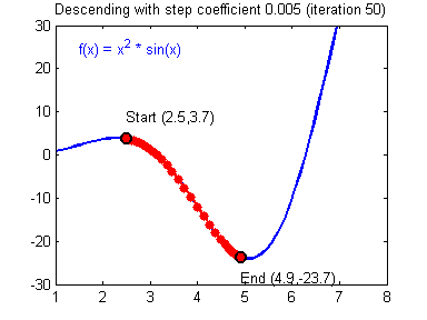
General gradient descent rule: $ \theta = \theta - \alpha \frac{\partial J }{ \partial \theta }$ where $\alpha$ is the learning rate and $\theta$ represents a parameter.

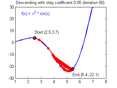
Illustration: The gradient descent algorithm with a good learning rate (converging) and a bad learning rate (diverging). Images courtesy of Adam Harley.

# GRADED FUNCTION: update_parameters

def update_parameters(parameters, grads, learning_rate = 1.2):
    """
    Updates parameters using the gradient descent update rule given above
    
    Arguments:
    parameters -- python dictionary containing your parameters 
    grads -- python dictionary containing your gradients 
    
    Returns:
    parameters -- python dictionary containing your updated parameters 
    """
    # Retrieve each parameter from the dictionary "parameters"
    ### START CODE HERE ### (≈ 4 lines of code)
    W1 = parameters['W1']
    b1 = parameters['b1']
    W2 = parameters['W2']
    b2 = parameters['b2']
    ### END CODE HERE ###
    
    # Retrieve each gradient from the dictionary "grads"
    ### START CODE HERE ### (≈ 4 lines of code)
    dW1 = grads['dW1']
    db1 = grads['db1']
    dW2 = grads['dW2']
    db2 = grads['db2']
    ## END CODE HERE ###
    
    # Update rule for each parameter
    ### START CODE HERE ### (≈ 4 lines of code)
    W1 -= learning_rate * dW1
    b1 -= learning_rate * db1
    W2 -= learning_rate * dW2
    b2 -= learning_rate * db2
    ### END CODE HERE ###
    
    parameters = {"W1": W1,
                  "b1": b1,
                  "W2": W2,
                  "b2": b2}
    
    return parameters

parameters, grads = update_parameters_test_case()
parameters = update_parameters(parameters, grads)

print("W1 = " + str(parameters["W1"]))
print("b1 = " + str(parameters["b1"]))
print("W2 = " + str(parameters["W2"]))
print("b2 = " + str(parameters["b2"]))

W1 = [[-0.00643025  0.01936718]
 [-0.02410458  0.03978052]
 [-0.01653973 -0.02096177]
 [ 0.01046864 -0.05990141]]
b1 = [[-1.02420756e-06]
 [ 1.27373948e-05]
 [ 8.32996807e-07]
 [-3.20136836e-06]]
W2 = [[-0.01041081 -0.04463285  0.01758031  0.04747113]]
b2 = [[0.00010457]]

Expected Output:

**W1**

[[-0.00643025 0.01936718] [-0.02410458 0.03978052] [-0.01653973 -0.02096177] [ 0.01046864 -0.05990141]]

**b1** [[ -1.02420756e-06] [ 1.27373948e-05] [ 8.32996807e-07] [ -3.20136836e-06]] **W2** [[-0.01041081 -0.04463285 0.01758031 0.04747113]] **b2** [[ 0.00010457]]

4.4 - Integrate parts 4.1, 4.2 and 4.3 in nn_model()

Question: Build your neural network model in nn_model().

Instructions: The neural network model has to use the previous functions in the right order.

# GRADED FUNCTION: nn_model

def nn_model(X, Y, n_h, num_iterations = 10000, print_cost=False):
    """
    Arguments:
    X -- dataset of shape (2, number of examples)
    Y -- labels of shape (1, number of examples)
    n_h -- size of the hidden layer
    num_iterations -- Number of iterations in gradient descent loop
    print_cost -- if True, print the cost every 1000 iterations
    
    Returns:
    parameters -- parameters learnt by the model. They can then be used to predict.
    """
    
    np.random.seed(3)
    n_x = layer_sizes(X, Y)[0]
    n_y = layer_sizes(X, Y)[2]
    
    # Initialize parameters, then retrieve W1, b1, W2, b2. Inputs: "n_x, n_h, n_y". Outputs = "W1, b1, W2, b2, parameters".
    ### START CODE HERE ### (≈ 5 lines of code)
    parameters = initialize_parameters(n_x, n_h, n_y)
    W1 = parameters['W1']
    b1 = parameters['b1']
    W2 = parameters['W2']
    b2 = parameters['b2']
    ### END CODE HERE ###
    
    # Loop (gradient descent)

    for i in range(0, num_iterations):
         
        ### START CODE HERE ### (≈ 4 lines of code)
        # Forward propagation. Inputs: "X, parameters". Outputs: "A2, cache".
        A2, cache = forward_propagation(X, parameters)
        
        # Cost function. Inputs: "A2, Y, parameters". Outputs: "cost".
        cost = compute_cost(A2, Y, parameters)
 
        # Backpropagation. Inputs: "parameters, cache, X, Y". Outputs: "grads".
        grads = backward_propagation(parameters, cache, X, Y)
 
        # Gradient descent parameter update. Inputs: "parameters, grads". Outputs: "parameters".
        parameters = update_parameters(parameters, grads)
        
        ### END CODE HERE ###
        
        # Print the cost every 1000 iterations
        if print_cost and i % 1000 == 0:
            print ("Cost after iteration %i: %f" %(i, cost))

    return parameters

X_assess, Y_assess = nn_model_test_case()

parameters = nn_model(X_assess, Y_assess, 4, num_iterations=10000, print_cost=False)
print("W1 = " + str(parameters["W1"]))
print("b1 = " + str(parameters["b1"]))
print("W2 = " + str(parameters["W2"]))
print("b2 = " + str(parameters["b2"]))

D:\Anaconda3\envs\Tensorflow\lib\site-packages\ipykernel_launcher.py:20: RuntimeWarning: divide by zero encountered in log
F:\PycharmProjects\DLcode\代码作业\第一课第三周编程作业\assignment3\planar_utils.py:34: RuntimeWarning: overflow encountered in exp
  s = 1/(1+np.exp(-x))


W1 = [[-4.18497897  5.33206142]
 [-7.53803882  1.20755762]
 [-4.19298806  5.32617188]
 [ 7.53798331 -1.20758933]]
b1 = [[ 2.32932918]
 [ 3.81001746]
 [ 2.33008879]
 [-3.81011387]]
W2 = [[-6033.8235662  -6008.1429712  -6033.08779759  6008.07951848]]
b2 = [[-52.67923259]]

Expected Output:

**W1**

[[-4.18494056 5.33220609] [-7.52989382 1.24306181] [-4.1929459 5.32632331] [ 7.52983719 -1.24309422]]

**b1** [[ 2.32926819] [ 3.79458998] [ 2.33002577] [-3.79468846]] **W2** [[-6033.83672146 -6008.12980822 -6033.10095287 6008.06637269]] **b2** [[-52.66607724]]

4.5 Predictions

Question: Use your model to predict by building predict().
Use forward propagation to predict results.

Reminder: predictions = $y_{prediction}=1\text{activation > 0.5}=\{\begin{array}{ll}1& \text{if}activation>0.5\\ 0& \text{otherwise}\end{array}$

As an example, if you would like to set the entries of a matrix X to 0 and 1 based on a threshold you would do: X_new = (X > threshold)

# GRADED FUNCTION: predict

def predict(parameters, X):
    """
    Using the learned parameters, predicts a class for each example in X
    
    Arguments:
    parameters -- python dictionary containing your parameters 
    X -- input data of size (n_x, m)
    
    Returns
    predictions -- vector of predictions of our model (red: 0 / blue: 1)
    """
    
    # Computes probabilities using forward propagation, and classifies to 0/1 using 0.5 as the threshold.
    ### START CODE HERE ### (≈ 2 lines of code)
    A2, cache = forward_propagation(X, parameters)
    predictions = np.around(A2)  # 四舍五入
    ### END CODE HERE ###
    
    return predictions

parameters, X_assess = predict_test_case()

predictions = predict(parameters, X_assess)
print("predictions mean = " + str(np.mean(predictions)))

predictions mean = 0.6666666666666666

​

Expected Output:

**predictions mean**

0.666666666667

It is time to run the model and see how it performs on a planar dataset. Run the following code to test your model with a single hidden layer of $n_h$ hidden units.

# Build a model with a n_h-dimensional hidden layer
parameters = nn_model(X, Y, n_h = 4, num_iterations = 10000, print_cost=True)

# Plot the decision boundary
plot_decision_boundary(lambda x: predict(parameters, x.T), X, Y)
plt.title("Decision Boundary for hidden layer size " + str(4))

Cost after iteration 0: 0.693048
Cost after iteration 1000: 0.288083
Cost after iteration 2000: 0.254385
Cost after iteration 3000: 0.233864
Cost after iteration 4000: 0.226792
Cost after iteration 5000: 0.222644
Cost after iteration 6000: 0.219731
Cost after iteration 7000: 0.217504
Cost after iteration 8000: 0.219460
Cost after iteration 9000: 0.218608





Text(0.5,1,'Decision Boundary for hidden layer size 4')

Expected Output:

**Cost after iteration 9000**

0.218607

# Print accuracy
predictions = predict(parameters, X)
print ('Accuracy: %d' % float((np.dot(Y,predictions.T) + np.dot(1-Y,1-predictions.T))/float(Y.size)*100) + '%')

Accuracy: 90%

​

Expected Output:

**Accuracy**

90%

Accuracy is really high compared to Logistic Regression. The model has learnt the leaf patterns of the flower! Neural networks are able to learn even highly non-linear decision boundaries, unlike logistic regression.

Now, let’s try out several hidden layer sizes.

4.6 - Tuning hidden layer size (optional/ungraded exercise)

Run the following code. It may take 1-2 minutes. You will observe different behaviors of the model for various hidden layer sizes.

# This may take about 2 minutes to run

plt.figure(figsize=(16, 32))
hidden_layer_sizes = [1, 2, 3, 4, 5, 10, 20]
for i, n_h in enumerate(hidden_layer_sizes):
    plt.subplot(5, 2, i+1)
    plt.title('Hidden Layer of size %d' % n_h)
    parameters = nn_model(X, Y, n_h, num_iterations = 5000)
    plot_decision_boundary(lambda x: predict(parameters, x.T), X, Y)
    predictions = predict(parameters, X)
    accuracy = float((np.dot(Y,predictions.T) + np.dot(1-Y,1-predictions.T))/float(Y.size)*100)
    print ("Accuracy for {} hidden units: {} %".format(n_h, accuracy))

Accuracy for 1 hidden units: 67.5 %
Accuracy for 2 hidden units: 67.25 %
Accuracy for 3 hidden units: 90.75 %
Accuracy for 4 hidden units: 90.5 %
Accuracy for 5 hidden units: 91.25 %
Accuracy for 10 hidden units: 90.25 %
Accuracy for 20 hidden units: 90.0 %

Interpretation:

• The larger models (with more hidden units) are able to fit the training set better, until eventually the largest models overfit the data.
• The best hidden layer size seems to be around n_h = 5. Indeed, a value around here seems to fits the data well without also incurring noticable overfitting.
• You will also learn later about regularization, which lets you use very large models (such as n_h = 50) without much overfitting.

Optional questions:

Note: Remember to submit the assignment but clicking the blue “Submit Assignment” button at the upper-right.

Some optional/ungraded questions that you can explore if you wish:

• What happens when you change the tanh activation for a sigmoid activation or a ReLU activation?
• Play with the learning_rate. What happens?
• What if we change the dataset? (See part 5 below!)

**You've learnt to:** - Build a complete neural network with a hidden layer - Make a good use of a non-linear unit - Implemented forward propagation and backpropagation, and trained a neural network - See the impact of varying the hidden layer size, including overfitting.

Nice work!

5) Performance on other datasets

If you want, you can rerun the whole notebook (minus the dataset part) for each of the following datasets.

# Datasets
noisy_circles, noisy_moons, blobs, gaussian_quantiles, no_structure = load_extra_datasets()

datasets = {"noisy_circles": noisy_circles,
            "noisy_moons": noisy_moons,
            "blobs": blobs,
            "gaussian_quantiles": gaussian_quantiles}

### START CODE HERE ### (choose your dataset)
dataset = "gaussian_quantiles"
### END CODE HERE ###

X, Y = datasets[dataset]
X, Y = X.T, Y.reshape(1, Y.shape[0])

# make blobs binary
if dataset == "blobs":
    Y = Y%2

# Visualize the data
plt.scatter(X[0, :], X[1, :], c=Y.flatten(), s=40, cmap=plt.cm.Spectral);

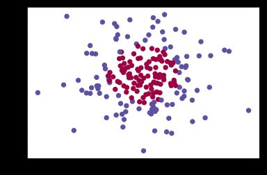[外链图片转存失败(img-KphV0H9w-1563354366315)(output_61_0.png)]

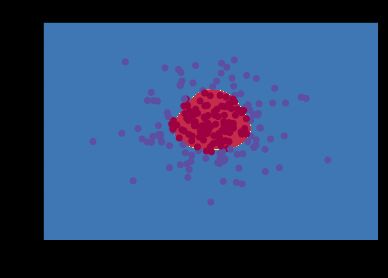
parameters = nn_model(X, Y, n_h = 3, num_iterations = 10000, print_cost=True)

# Plot the decision boundary
plot_decision_boundary(lambda x: predict(parameters, x.T), X, Y)
plt.title("Decision Boundary for hidden layer size " + str(4))

Cost after iteration 0: 0.693147
Cost after iteration 1000: 0.134908
Cost after iteration 2000: 0.127436
Cost after iteration 3000: 0.128161
Cost after iteration 4000: 0.128443
Cost after iteration 5000: 0.101724
Cost after iteration 6000: 0.135567
Cost after iteration 7000: 0.115572
Cost after iteration 8000: 0.095704
Cost after iteration 9000: 0.123006





Text(0.5,1,'Decision Boundary for hidden layer size 4')