R语言绘图——Graphics包
先给出一下参考说明:
R绘图 http://www.cnblogs.com/holbrook/archive/2013/05/13/3075777.html
R语言中颜色对照表 http://wenku.baidu.com/link?url=PnCsIjv3e_OGw2COt4AEo3_tHTisOYoHLGf9bf-jjzkfGIJhFZpEQrS6CAELUypnR82Wdj6VclURzzACwbUOszZVHoPnNt27RiM-Uv1B4z3
参考书《R语言核心技术手册》
我只是个勤劳的搬运工,主要是根据上面说到的参考书中的例子或者是说明文档中的例子,加以整理,放在这里,总结也是个自己以后的一个备份。
Graphic包常见的可绘制的图
| Graphic中的函数 |
描述 |
说明文档 |
| plot |
画图基础函数,可绘制多种图,用type参数控制图的类型 |
http://127.0.0.1:10143/library/graphics/html/plot.html |
| matplot |
类似plot可画多种图,同时展示多列数据 |
http://127.0.0.1:10143/library/graphics/html/matplot.html |
| barplot |
柱状图或列图 |
http://127.0.0.1:10143/library/graphics/html/barplot.html |
| dotchart |
克利夫兰点图 |
http://127.0.0.1:10143/library/graphics/html/dotchart.html |
| hist |
直方图 |
http://127.0.0.1:10143/library/graphics/html/hist.html |
| pie |
饼图 |
http://127.0.0.1:10143/library/graphics/html/pie.html |
| density |
核密度图 |
http://127.0.0.1:10143/library/stats/html/density.html |
| stripchart |
纸带图 |
http://127.0.0.1:10143/library/graphics/html/stripchart.html |
| smoothScatter |
平滑散点图 |
http://127.0.0.1:10143/library/graphics/html/smoothScatter.html |
| pairs |
散点矩阵图 |
http://127.0.0.1:10143/library/graphics/html/pairs.html |
| image |
image图 |
http://127.0.0.1:10143/doc/html/Search?pattern=image |
| contour |
等高图 |
http://127.0.0.1:10143/library/graphics/html/contour.html |
| persp |
三维数据透视图 |
http://127.0.0.1:10143/library/graphics/html/persp.html |
| heatmap(stats中) |
热图 |
http://127.0.0.1:10143/library/stats/html/heatmap.html |
| sunflowerplot |
太阳花图 |
http://127.0.0.1:10143/library/graphics/html/sunflowerplot.html |
数据导入(主要数据来自nutshell包)
require(“nutshell”)
library(nutshell)
plot()
data(toxins.and.cancer)
attach(toxins.and.cancer)
plot(total_toxic_chemicals/Surface_Area,deaths_total/Population)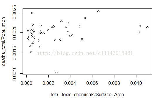
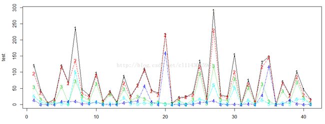
matplot()
test <-toxins.and.cancer[,c(-1,-7,-8,-9,-10,-11,-12,-13,-14,-15)]
colnames(test)
[1]"total_toxic_chemicals"
[2] "total_on_site"
[3] "air_on_site"
[4] "other_on_site"
[5] "off_site"
matplot(test)
matplot(test,type='l')
matplot(test,type='o')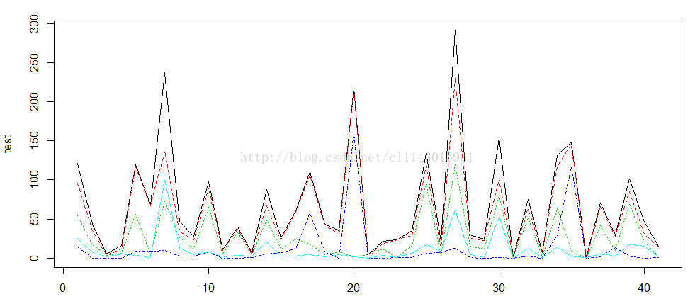
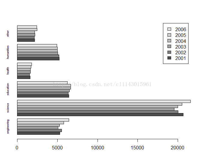
barplot()
data(doctorates)
doctorates
doctorates.m <-as.matrix(doctorates[2:7])
rownames(doctorates.m) <-doctorates[,1]
barplot(doctorates.m,legend=TRUE)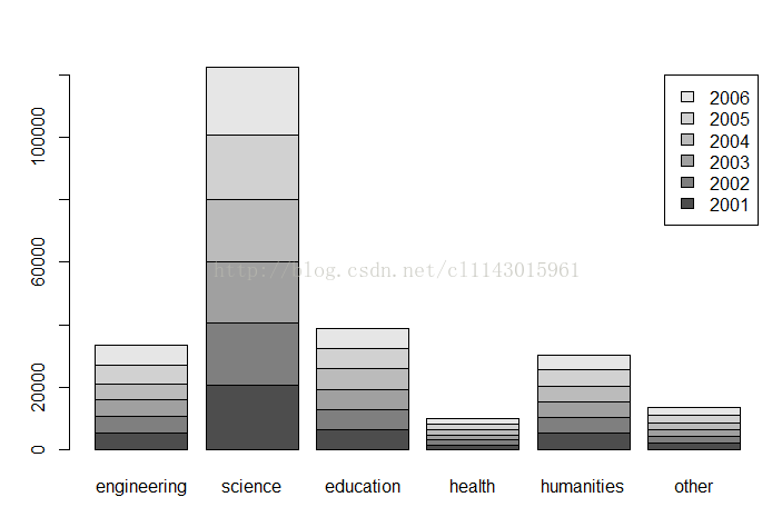
barplot(doctorates.m,beside=TRUE,horiz=TRUE,legend=TRUE,cex.names=.75)
barplot(doctorates.m,beside=TRUE,horiz=TRUE,legend=TRUE,cex.names=.55)#y轴字体的大小
barplot(doctorates.m,beside=TRUE,horiz=TRUE,legend=TRUE,cex.names=.55,col=c("yellow","gray","orange","blue","red","purple"))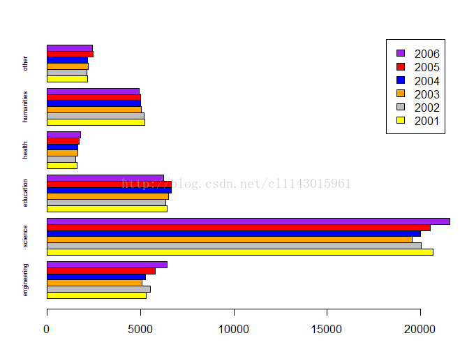
barplot(t(doctorates.m),legend=TRUE,ylim=c(0,66000))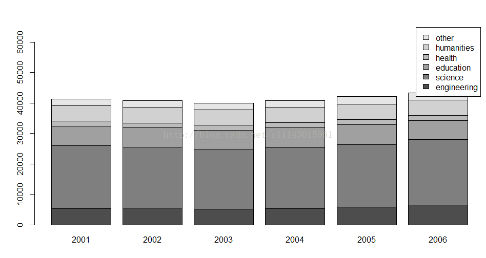
pie()
domestic.catch.2006 <-c(7752,1166,463,108)
names(domestic.catch.2006) <-c("one","two","three","four")
pie(domestic.catch.2006,init.angle=90)
pie(domestic.catch.2006,init.angle=100,main="捕鱼数据",sub="单位:百万磅")
persp()
data(yosemite)
dim(yosemit)
dim(yosemite)
[1] 562 253
yosemite.flipped <-yosemite[,seq(from=253,to=1)]
yosemite.rightmost <-yosemite[nrow(yosemite)-ncol(yosemite)+1,]
halfdome <-yosemite[(nrow(yosemite)-ncol(yosemite)+1):562,seq(from=253,to=1)]
persp(halfdome,col=gray(.15),border=NA,expand=.15,theta=225,phi=20,ltheta=45,lphi=20,shade=.55)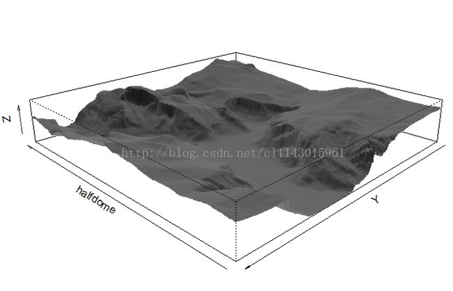
image()
image(yosemite,asp=253/562,ylim=c(1,0),col=sapply((0:32)/32,gray))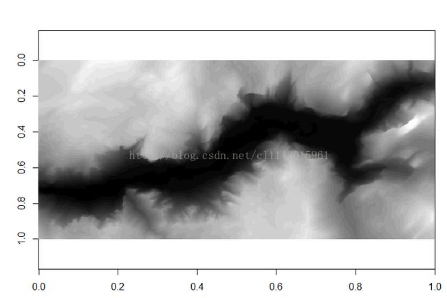
contour()
contour(yosemite,asp=253/562,ylim=c(1,0))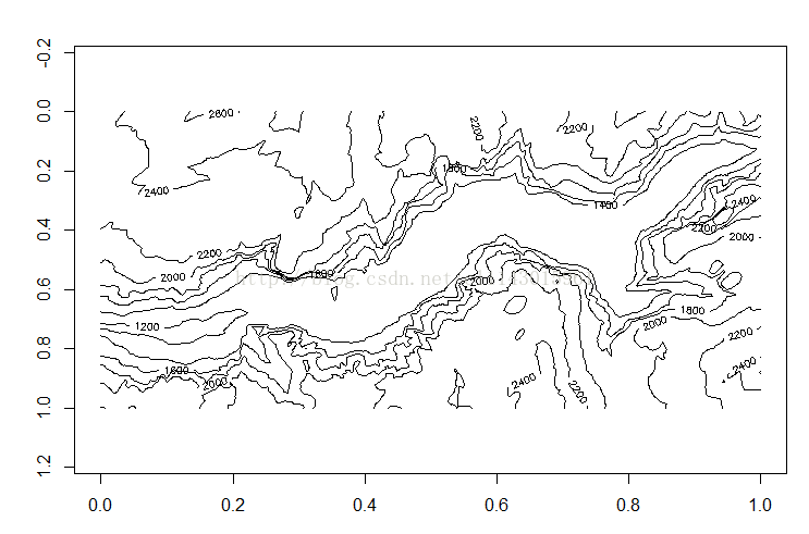
heatmap()
参考文章http://my.oschina.net/u/1791586/blog/285250,下面例子是说明文档中的一个最简单的例子。
x <- as.matrix(mtcars)
rc <- rainbow(nrow(x), start = 0,end = .3)
cc <- rainbow(ncol(x), start = 0,end = .3)
hv <- heatmap(x, col =cm.colors(256), scale = "column",
+               RowSideColors = rc,ColSideColors = cc, margins = c(5,10),
+               xlab = "specificationvariables", ylab =  "CarModels",
+               main = "heatmap(, ..., scale = \"column\")")
utils::str(hv) # the two re-orderingindex vectors
List of 4
 $ rowInd: int [1:32] 31 17 16 15 5 25 29 24 76 ...
 $ colInd: int [1:11] 2 9 8 11 6 5 10 7 1 4 ...
 $ Rowv : NULL
$ Colv : NULL 