机器学习之机器学习库scikit-learn

一、 加载sklearn中的数据集datasets

from sklearn import datasets

iris = datasets.load_iris() # 鸢尾花卉数据
digits = datasets.load_digits() # 手写数字8x8像素信息数据

• 查看数据的信息

print iris.data[:4] # 查看数据的特征信息
print iris.data.shape # 查看数据的特征信息维度

print iris.target_names # 查看标签对应的文本
print iris.target[:4] # 查看数据的标签 setosa:0 ...

    [[ 5.1  3.5  1.4  0.2]
     [ 4.9  3.   1.4  0.2]
     [ 4.7  3.2  1.3  0.2]
     [ 4.6  3.1  1.5  0.2]]
    (150L, 4L)
    ['setosa' 'versicolor' 'virginica']
    [0 0 0 0]

print digits.data.shape
print digits.target[0]
print digits.data[0].reshape((8,8)) # 重塑成8x8的像素数组

    (1797L, 64L)
    0
    [[  0.   0.   5.  13.   9.   1.   0.   0.]
     [  0.   0.  13.  15.  10.  15.   5.   0.]
     [  0.   3.  15.   2.   0.  11.   8.   0.]
     [  0.   4.  12.   0.   0.   8.   8.   0.]
     [  0.   5.   8.   0.   0.   9.   8.   0.]
     [  0.   4.  11.   0.   1.  12.   7.   0.]
     [  0.   2.  14.   5.  10.  12.   0.   0.]
     [  0.   0.   6.  13.  10.   0.   0.   0.]]

二、训练集和分割集的分割

from sklearn.model_selection import train_test_split

X = digits.data # 特征矩阵
y = digits.target # 标签向量

# 随机分割训练集和测试集：
# test_size：设置测试集的比例。random_state:可理解为种子，保证随机唯一
X_train, X_test, y_train, y_test = train_test_split(X, y, test_size=1/3., random_state=8) 

print X_train.shape
print X_test.shape

(1198L, 64L)
(599L, 64L)

三、数据预处理

1. 缺失值处理

from sklearn.preprocessing import Imputer

x = np.array([[ 1, 2 , 0],
             [0, np.NaN,0],
             [0, 0, 1]]);

imputer = Imputer(missing_values='NaN',strategy='mean',axis=0,copy=False)
imputer.fit_transform(x[:,1])

array([[ 1.,  2.,  0.],
       [ 0.,  1.,  0.],
       [ 0.,  0.,  1.]])

2. 特征值的归一化

归一化的好处：

• 当特征的数值范围差距较大时，需要对特征的数值进行标准化，防止某些特征的权重过大，让每个特征的地位相对平等，对结果做出的贡献相同。一般对连续性特征值处理。

• 提升模型的收敛速度（梯度下降）。

from sklearn import preprocessing
import numpy as np

X = np.array([[1., -1., 2.],
              [2., 0., 0.],
              [0., 1., -1.]])


# 对每一列特征的数值归一化（均值为0，方差为1）
print preprocessing.scale(X)

array([[ 0.        , -1.22474487,  1.33630621],
       [ 1.22474487,  0.        , -0.26726124],
       [-1.22474487,  1.22474487, -1.06904497]])

• 使用StandardScaler对象进行归一化

  StandardScaler对象可以保存训练集中的参数（均值、方差），之后可以直接使用其对象转换测试集数据。

from sklearn.preprocessing import StandardScaler # 对数据标准

scaler = StandardScaler()
X_std_train = scaler.fit_transform(X_train)
X_std_test = scaler.transform(X_test)

• 其他预处理：

# : 区间缩放
from sklearn.preprocessing import MinMaxScaler
# : 归一化
from sklearn.preprocessing import Normalizer
# : 二值化（大于阈值的为1，小于等于则为0）
from sklearn.preprocessing import Binarizer

• 验证归一化的重要性

# 生成分类数据进行验证
from sklearn import datasets
import matplotlib.pyplot as plt
%matplotlib inline

# 生成分类数据：
# n_sample:样本个数、n_features:类别标签种类数
X, y = datasets.make_classification(n_samples=300, n_features=2, n_redundant=0, n_informative=2, 
                           random_state=25, n_clusters_per_class=1, scale=100)

plt.scatter(X[:,0], X[:,1], c=y)
plt.show()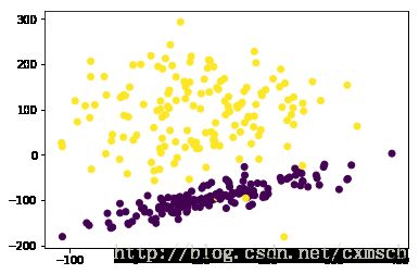

• 使用svm模型（未特征归一化时）

# 使用svm模型（未特征归一化时）
from sklearn import svm

# X = preprocessing.scale(X)

# 分割训练集合测试集
X_train, X_test, y_train, y_test = train_test_split(X, y, test_size=1/3., random_state=7) 

svm_classifier = svm.SVC()

# 训练模型
svm_classifier.fit(X_train, y_train)

# 在测试集上对模型打分
svm_classifier.score(X_test, y_test)

0.52000000000000002

• 使用svm模型（特征归一化时）

# 使用svm模型（特征归一化时）
from sklearn import svm

X = preprocessing.scale(X)

# 分割训练集合测试集
X_train, X_test, y_train, y_test = train_test_split(X, y, test_size=1/3., random_state=7) 

svm_classifier = svm.SVC()
svm_classifier.fit(X_train, y_train)
svm_classifier.score(X_test, y_test)

0.97999999999999998

3. 特征值的编码

• 将字符串类型的类别名转化为整型：

from sklearn.preprocessing import LabelEncoder

x = np.array(['A','B','C','B'])
encoding = LabelEncoder()
print encoding.fit_transform(x)

[0 1 2 1]

y = np.array(['A','C'])
print encoding.transform(y)

[0 2]

- 一值化：将一维（类别）特征转化为多维特征的表示

from sklearn.preprocessing import OneHotEncoder

onehot = OneHotEncoder()
x = np.array([[0],[1],[2]])
print onehot.fit_transform(x).todense()

[[ 1.  0.  0.]
 [ 0.  1.  0.]
 [ 0.  0.  1.]]

import pandas as pd
x = np.array(['A','B','C'])
pd.get_dummies(x,prefix='class')

	class_A	class_B	class_C
0	1	0	0
1	0	1	0
2	0	0	1

四、模型的训练、预测与保存

• 以线性回归模型为例

iris = datasets.load_iris() # 鸢尾花卉数据

X = iris.data
y = iris.target
print X[:3]
print y[:3]

[[ 5.1  3.5  1.4  0.2]
 [ 4.9  3.   1.4  0.2]
 [ 4.7  3.2  1.3  0.2]]
[0 0 0]

# 选择线性回归模型
from sklearn.linear_model import LinearRegression

# 新建一个模型(参数默认)
iris_model = LinearRegression()

# 分割训练集、测试集
X_train, X_test, y_train, y_test = train_test_split(X, y, test_size=1/3., random_state=7) 

# 训练该模型
iris_model.fit(X_train,y_train)

# 返回模型参数列表
iris_model.get_params()

{'copy_X': True, 'fit_intercept': True, 'n_jobs': 1, 'normalize': False}

# 模型在训练集上的评分
iris_model.score(X_train, y_train)

0.94505820275667418

# 模型在测试集上的评分
iris_model.score(X_test, y_test)

0.89618390663189063

# 使用模型进行预测
y_pred = iris_model.predict(X_test)

print '预测标签：', y_pred[:3]
print '真实标签：', y_test[:3]

预测标签： [ 1.66080893  1.39414184 -0.02450645]
真实标签： [2 1 0]

# 使用pickle保存模型

import cPickle as pickle

with open('LR_model.pkl', 'w') as f:
    pickle.dump(iris_model, f)

# 重新加载模型进行预测
with open('LR_model.pkl', 'r') as f:
    model = pickle.load(f)

# 使用模型进行预测
model.predict(X_test)[:3]

array([ 1.66080893,  1.39414184, -0.02450645])

五、交叉验证

在分割训练集和测试集后，测试集一般用于对最后选择的模型进行评分。而在选择模型的超参数的过程中，为验证/评价模型的好坏，需要在训练集中取出一定比例的样本作为验证集来评价某个模型的好坏，训练集中的其他样本用来训练模型。

为消除所选出来的验证集中的样本的特殊性，则需要将训练集中的每一份样本作为验证集，其他样本作为训练集来训练模型。若将训练集中的样本分为N分，最后会得到N个对该模型的评分，对这些评分取均值，即得到了交叉验证的评分。

交叉验证一般用来调整模型的超参数。

• sklearn中的交叉验证

  cross_val_score函数用于交叉验证，返回各个验证集的评价得分。

from sklearn import datasets
from sklearn.model_selection import train_test_split
from sklearn.model_selection import cross_val_score
import matplotlib.pyplot as plt
%matplotlib inline

iris = datasets.load_iris()
X = iris.data
y = iris.target

X_train, X_test, y_train, y_test = train_test_split(X, y, test_size=1/3., random_state=5)

• 以KNN模型为例

# 使用KNN模型进行预测（K为超参数）
from sklearn.neighbors import KNeighborsClassifier

# 超参数K的范围
k_range = range(1,31)

# 交叉验证的评分集合
cv_scores = []

for k in k_range:
    knn = KNeighborsClassifier(k) # 构造模型
    # 将训练集均分为10份
    #cv: 交叉验证迭代器
    scores = cross_val_score(knn, X_train, y_train, cv=10, scoring='accuracy') # 分类问题使用
    #scores = cross_val_score(knn, X_train, y_train, cv=10, scoring='neg_mean_squared_error') # 回归问题使用
    cv_scores.append(scores.mean()) # 

# print cv_scores
# 可视化各个k值模型的交叉验证的平均分
plt.plot(k_range,cv_scores)
plt.xlabel('k')
plt.ylabel('Accuracy')
plt.show()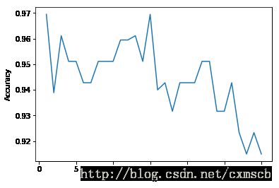

# 选择最优的超参数K

best_knn = KNeighborsClassifier(15)
best_knn.fit(X_train, y_train)
print best_knn.score(X_test, y_test)

1.0

• 网格搜索：GridSearchCV

from sklearn.datasets import load_digits
from sklearn.ensemble import RandomForestClassifier
from sklearn.model_selection import GridSearchCV

digits = load_digits()
params = {'n_estimators':(1000,2000),
          'criterion':('gini','entropy'),
          'min_samples_leaf':(1,2,3)
         }
clf = GridSearchCV(RandomForestClassifier(),param_grid=params)
clf.fit(digits.data,digits.target)
print clf.score(digits.data,digits.target)
print clf.get_params()
print clf.best_estimator_

1.0
RandomForestClassifier(bootstrap=True, class_weight=None, criterion='gini',
            max_depth=None, max_features='auto', max_leaf_nodes=None,
            min_impurity_split=1e-07, min_samples_leaf=1,
            min_samples_split=2, min_weight_fraction_leaf=0.0,
            n_estimators=2000, n_jobs=1, oob_score=False,
            random_state=None, verbose=0, warm_start=False)

六、过拟合与欠拟合

过拟合：模型对于训练集数据拟合程度过当，以致太适合训练集数据而无法适应一般情况。即训练出来的模型在训练集上表现很好，在验证集/测试集上表现并不好。

欠拟合：模型在训练集/测试集上都表现得不是很好。

# 加载数据
from sklearn.model_selection import learning_curve
from sklearn.svm import SVC
import numpy as np

digits = datasets.load_digits()
X = digits.data
y = digits.target

• 欠拟合情况

# 绘制学习曲线（学习曲线：在不同训练数据量下对训练出来的模型进行评分）
# gamma = 0.001
train_sizes, train_scores, val_scores = learning_curve(
    SVC(gamma=0.001), X, y, cv=10, scoring='accuracy',
    train_sizes=[0.1, 0.25, 0.5, 0.75, 1]
)
# train_sizes: 每次模型训练的数量
# train_scores: 每次模型在训练集上的评分
# val_scores：每次模型在验证集上的交叉验证评分

# 求不同训练数据量下的评分的均值
train_scores_mean = np.mean(train_scores, axis=1) # 行均值
val_scores_mean = np.mean(val_scores, axis=1)

# 绘制学习曲线
plt.plot(train_sizes, train_scores_mean, 'o-', color='r', label='training')
plt.plot(train_sizes, val_scores_mean, '*-', color='g', label='cross validation')

plt.xlabel('training sample size')
plt.ylabel('accuracy')
plt.legend(loc='best')
plt.show()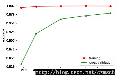

如图所示：当训练数据量较少时，模型在交叉验证中的得分较低，可看作一种欠拟合现象；随着训练数据量的增多，交叉验证的平均分也随之增加

• 过拟合

train_sizes, train_scores, val_scores = learning_curve(
            SVC(gamma=0.1), X, y, cv=10, scoring='accuracy',
            train_sizes=[0.1, 0.25, 0.5, 0.75, 1]
            )

# 求不同训练数据量下的评分的均值
train_scores_mean = np.mean(train_scores, axis=1) # 行均值
val_scores_mean = np.mean(val_scores, axis=1)

# 绘制学习曲线
plt.plot(train_sizes, train_scores_mean, 'o-', color='r', label='training')
plt.plot(train_sizes, val_scores_mean, '*-', color='g', label='cross validation')

plt.xlabel('training sample size')
plt.ylabel('accuracy')
plt.legend(loc='best')
plt.show()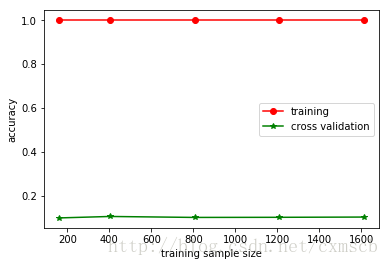

 如图所示：当训练数据量较少时，模型在交叉验证中的得分较低；然而，随着训练数据量的增多，交叉验证的平均分并没增多。因此出现过拟合现象。

• 通过验证曲线来观察过拟合

# 绘制验证曲线（验证曲线：在不同超参数下对模型的评分）
from sklearn.model_selection import validation_curve

# 设置SVC模型的超参数gamma的取值范围
gamma_range = np.arange(1, 10) / 3000.

train_scores, val_scores = validation_curve(
    SVC(), X, y, param_name='gamma', param_range=gamma_range,
    cv=5, scoring='accuracy')

# train_scores: 每次模型在训练集上的评分
# val_scores：每次模型在验证集上的交叉验证评分

# 求每次的平均值
train_scores_mean = np.mean(train_scores, axis=1)
val_scores_mean = np.mean(val_scores, axis=1)

# 绘制验证曲线
plt.plot(gamma_range, train_scores_mean, 'o-', color='r', label='training')
plt.plot(gamma_range, val_scores_mean, '*-', color='g', label='cross validation')

plt.xlabel('gamma')
plt.ylabel('accuracy')
plt.legend(loc='best')
plt.show()

如图所示：当gamma>0.0015时，出现过拟合现象，对应模型在训练集上的评分不断增大，而在验证集上的评分反而在减小