cs231 Network Visualization (PyTorch)

cs231 Network Visualization (PyTorch)

在本笔记本中，我们将探索使用图像梯度来生成新图像。

在训练模型时，我们定义一个损失函数，用来测量我们当前对模型性能的损失程度，使用反向传播来计算损失相对于模型参数的梯度，并对模型参数执行梯度下降来最小化损失。在这里，我们会做一些稍微不同的事情。我们将从卷积神经网络模型开始，该模型已经被预训练用于对ImageNet数据集执行图像分类。我们将使用这个模型来定义一个损失函数，它量化我们当前对图像的损失度，然后使用反向传播来计算这个损失相对于图像的像素的梯度。然后，我们将保持模型固定，并对图像执行梯度下降以合成新图像，使损失最小化。

在本笔记本中，我们将探讨三种用于图像生成的技术：
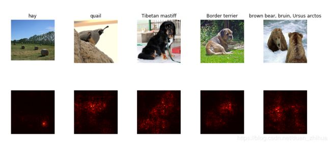
-Saliency Maps：Saliency Maps是一种快速方法，用来判断图像的哪个部分影响网络做出的分类决策。

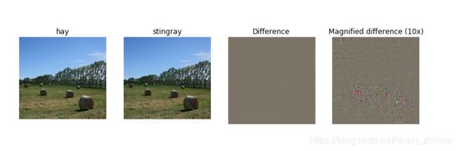
-Fooling Images：我们可以干扰输入图像，使其看起来与人类观察的图片一样，但会被预先训练的网络误分类。

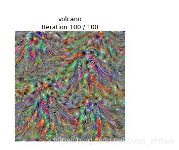
-分类可视化：我们可以合成一个图像来最大化一个特定类的分类分数；这可以让我们知道当网络对那个类的图像进行分类时，它在寻找什么。本笔记本使用PyTorch。

# -*- coding: utf-8 -*-

import torch
import torchvision
import torchvision.transforms as T
import random
import numpy as np
from scipy.ndimage.filters import gaussian_filter1d
import matplotlib.pyplot as plt
from cs231n.image_utils import SQUEEZENET_MEAN, SQUEEZENET_STD
from PIL import Image

#%matplotlib inline
plt.rcParams['figure.figsize'] = (10.0, 8.0) # set default size of plots
plt.rcParams['image.interpolation'] = 'nearest'
plt.rcParams['image.cmap'] = 'gray'



def preprocess(img, size=224):
    transform = T.Compose([
        T.Resize(size),
        T.ToTensor(),
        T.Normalize(mean=SQUEEZENET_MEAN.tolist(),
                    std=SQUEEZENET_STD.tolist()),
        T.Lambda(lambda x: x[None]),
    ])
    return transform(img)

def deprocess(img, should_rescale=True):
    transform = T.Compose([
        T.Lambda(lambda x: x[0]),
        T.Normalize(mean=[0, 0, 0], std=(1.0 / SQUEEZENET_STD).tolist()),
        T.Normalize(mean=(-SQUEEZENET_MEAN).tolist(), std=[1, 1, 1]),
        T.Lambda(rescale) if should_rescale else T.Lambda(lambda x: x),
        T.ToPILImage(),
    ])
    return transform(img)

def rescale(x):
    low, high = x.min(), x.max()
    x_rescaled = (x - low) / (high - low)
    return x_rescaled
    
def blur_image(X, sigma=1):
    X_np = X.cpu().clone().numpy()
    X_np = gaussian_filter1d(X_np, sigma, axis=2)
    X_np = gaussian_filter1d(X_np, sigma, axis=3)
    X.copy_(torch.Tensor(X_np).type_as(X))
    return X


# Download and load the pretrained SqueezeNet model.
model = torchvision.models.squeezenet1_1(pretrained=True)

# We don't want to train the model, so tell PyTorch not to compute gradients
# with respect to model parameters.
for param in model.parameters():
    param.requires_grad = False
    
# you may see warning regarding initialization deprecated, that's fine, please continue to next steps
    
    
    
from cs231n.data_utils import load_imagenet_val
X, y, class_names = load_imagenet_val(num=5)

plt.figure(figsize=(12, 6))
for i in range(5):
    plt.subplot(1, 5, i + 1)
    plt.imshow(X[i])
    plt.title(class_names[y[i]])
    plt.axis('off')
plt.gcf().tight_layout()    



# Example of using gather to select one entry from each row in PyTorch
def gather_example():
    N, C = 4, 5
    s = torch.randn(N, C)
    y = torch.LongTensor([1, 2, 1, 3])
    print(s)
    print(y)
    print(s.gather(1, y.view(-1, 1)).squeeze())
gather_example()

def compute_saliency_maps(X, y, model):
    """
    Compute a class saliency map using the model for images X and labels y.

    Input:
    - X: Input images; Tensor of shape (N, 3, H, W)
    - y: Labels for X; LongTensor of shape (N,)
    - model: A pretrained CNN that will be used to compute the saliency map.

    Returns:
    - saliency: A Tensor of shape (N, H, W) giving the saliency maps for the input
    images.
    """
    # Make sure the model is in "test" mode
    model.eval()
    
    # Make input tensor require gradient
    X.requires_grad_()
    
    saliency = None
    ##############################################################################
    # TODO: Implement this function. Perform a forward and backward pass through #
    # the model to compute the gradient of the correct class score with respect  #
    # to each input image. You first want to compute the loss over the correct   #
    # scores (we'll combine losses across a batch by summing), and then compute  #
    # the gradients with a backward pass.                                        #
    ##############################################################################
    scores = model(X)
    scores = scores.gather(1, y.view(-1, 1))
    scores.backward(torch.ones_like(scores))
    saliency = X.grad.data.abs().max(1)[0]
    ##############################################################################
    #                             END OF YOUR CODE                               #
    ##############################################################################
    return saliency



def show_saliency_maps(X, y):
    # Convert X and y from numpy arrays to Torch Tensors
    X_tensor = torch.cat([preprocess(Image.fromarray(x)) for x in X], dim=0)
    y_tensor = torch.LongTensor(y)

    # Compute saliency maps for images in X
    saliency = compute_saliency_maps(X_tensor, y_tensor, model)

    # Convert the saliency map from Torch Tensor to numpy array and show images
    # and saliency maps together.
    saliency = saliency.numpy()
    N = X.shape[0]
    for i in range(N):
        plt.subplot(2, N, i + 1)
        plt.imshow(X[i])
        plt.axis('off')
        plt.title(class_names[y[i]])
        plt.subplot(2, N, N + i + 1)
        plt.imshow(saliency[i], cmap=plt.cm.hot)
        plt.axis('off')
        plt.gcf().set_size_inches(12, 5)
    plt.show()

show_saliency_maps(X, y)






def make_fooling_image(X, target_y, model):
    """
    Generate a fooling image that is close to X, but that the model classifies
    as target_y.

    Inputs:
    - X: Input image; Tensor of shape (1, 3, 224, 224)
    - target_y: An integer in the range [0, 1000)
    - model: A pretrained CNN

    Returns:
    - X_fooling: An image that is close to X, but that is classifed as target_y
    by the model.
    """
    # Initialize our fooling image to the input image, and make it require gradient
    X_fooling = X.clone()
    X_fooling = X_fooling.requires_grad_()
    
    learning_rate = 1
    ##############################################################################
    # TODO: Generate a fooling image X_fooling that the model will classify as   #
    # the class target_y. You should perform gradient ascent on the score of the #
    # target class, stopping when the model is fooled.                           #
    # When computing an update step, first normalize the gradient:               #
    #   dX = learning_rate * g / ||g||_2                                         #
    #                                                                            #
    # You should write a training loop.                                          #
    #                                                                            #
    # HINT: For most examples, you should be able to generate a fooling image    #
    # in fewer than 100 iterations of gradient ascent.                           #
    # You can print your progress over iterations to check your algorithm.       #
    ##############################################################################
    for i in range(100):
        scores = model(X_fooling)
        if scores.argmax(1)[0] == target_y:
            break
        scores = scores[:, target_y]
        scores.backward()
        dx = X_fooling.grad.data
        dx = learning_rate * dx / torch.norm(dx)
        X_fooling.data += dx
        X_fooling.grad.zero_()
    ##############################################################################
    #                             END OF YOUR CODE                               #
    ##############################################################################
    return X_fooling


idx = 0
target_y = 6

X_tensor = torch.cat([preprocess(Image.fromarray(x)) for x in X], dim=0)
X_fooling = make_fooling_image(X_tensor[idx:idx+1], target_y, model)

scores = model(X_fooling)
assert target_y == scores.data.max(1)[1][0].item(), 'The model is not fooled!'




X_fooling_np = deprocess(X_fooling.clone())
X_fooling_np = np.asarray(X_fooling_np).astype(np.uint8)

plt.subplot(1, 4, 1)
plt.imshow(X[idx])
plt.title(class_names[y[idx]])
plt.axis('off')

plt.subplot(1, 4, 2)
plt.imshow(X_fooling_np)
plt.title(class_names[target_y])
plt.axis('off')

plt.subplot(1, 4, 3)
X_pre = preprocess(Image.fromarray(X[idx]))
diff = np.asarray(deprocess(X_fooling - X_pre, should_rescale=False))
plt.imshow(diff)
plt.title('Difference')
plt.axis('off')

plt.subplot(1, 4, 4)
diff = np.asarray(deprocess(10 * (X_fooling - X_pre), should_rescale=False))
plt.imshow(diff)
plt.title('Magnified difference (10x)')
plt.axis('off')

plt.gcf().set_size_inches(12, 5)
plt.show()




def jitter(X, ox, oy):
    """
    Helper function to randomly jitter an image.
    
    Inputs
    - X: PyTorch Tensor of shape (N, C, H, W)
    - ox, oy: Integers giving number of pixels to jitter along W and H axes
    
    Returns: A new PyTorch Tensor of shape (N, C, H, W)
    """
    if ox != 0:
        left = X[:, :, :, :-ox]
        right = X[:, :, :, -ox:]
        X = torch.cat([right, left], dim=3)
    if oy != 0:
        top = X[:, :, :-oy]
        bottom = X[:, :, -oy:]
        X = torch.cat([bottom, top], dim=2)
    return X


def create_class_visualization(target_y, model, dtype, **kwargs):
    """
    Generate an image to maximize the score of target_y under a pretrained model.
    
    Inputs:
    - target_y: Integer in the range [0, 1000) giving the index of the class
    - model: A pretrained CNN that will be used to generate the image
    - dtype: Torch datatype to use for computations
    
    Keyword arguments:
    - l2_reg: Strength of L2 regularization on the image
    - learning_rate: How big of a step to take
    - num_iterations: How many iterations to use
    - blur_every: How often to blur the image as an implicit regularizer
    - max_jitter: How much to gjitter the image as an implicit regularizer
    - show_every: How often to show the intermediate result
    """
    model.type(dtype)
    l2_reg = kwargs.pop('l2_reg', 1e-3)
    learning_rate = kwargs.pop('learning_rate', 25)
    num_iterations = kwargs.pop('num_iterations', 100)
    blur_every = kwargs.pop('blur_every', 10)
    max_jitter = kwargs.pop('max_jitter', 16)
    show_every = kwargs.pop('show_every', 25)

    # Randomly initialize the image as a PyTorch Tensor, and make it requires gradient.
    img = torch.randn(1, 3, 224, 224).mul_(1.0).type(dtype).requires_grad_()

    for t in range(num_iterations):
        # Randomly jitter the image a bit; this gives slightly nicer results
        ox, oy = random.randint(0, max_jitter), random.randint(0, max_jitter)
        img.data.copy_(jitter(img.data, ox, oy))

        ########################################################################
        # TODO: Use the model to compute the gradient of the score for the     #
        # class target_y with respect to the pixels of the image, and make a   #
        # gradient step on the image using the learning rate. Don't forget the #
        # L2 regularization term!                                              #
        # Be very careful about the signs of elements in your code.            #
        ########################################################################
        scores = model(img)
        scores = scores[:, target_y]
        scores.backward()
        dx = img.grad.data + 2 * l2_reg * img.data
        img.data += learning_rate * (dx / torch.norm(dx))
        img.grad.zero_()
        ########################################################################
        #                             END OF YOUR CODE                         #
        ########################################################################
        
        # Undo the random jitter
        img.data.copy_(jitter(img.data, -ox, -oy))

        # As regularizer, clamp and periodically blur the image
        for c in range(3):
            lo = float(-SQUEEZENET_MEAN[c] / SQUEEZENET_STD[c])
            hi = float((1.0 - SQUEEZENET_MEAN[c]) / SQUEEZENET_STD[c])
            img.data[:, c].clamp_(min=lo, max=hi)
        if t % blur_every == 0:
            blur_image(img.data, sigma=0.5)
        
        # Periodically show the image
        if t == 0 or (t + 1) % show_every == 0 or t == num_iterations - 1:
            plt.imshow(deprocess(img.data.clone().cpu()))
            class_name = class_names[target_y]
            plt.title('%s\nIteration %d / %d' % (class_name, t + 1, num_iterations))
            plt.gcf().set_size_inches(4, 4)
            plt.axis('off')
            plt.show()

    return deprocess(img.data.cpu())

dtype = torch.FloatTensor
# dtype = torch.cuda.FloatTensor # Uncomment this to use GPU
model.type(dtype)

target_y = 76 # Tarantula
# target_y = 78 # Tick
# target_y = 187 # Yorkshire Terrier
# target_y = 683 # Oboe
# target_y = 366 # Gorilla
# target_y = 604 # Hourglass
out = create_class_visualization(target_y, model, dtype)



# target_y = 78 # Tick
# target_y = 187 # Yorkshire Terrier
# target_y = 683 # Oboe
# target_y = 366 # Gorilla
# target_y = 604 # Hourglass
target_y = np.random.randint(1000)
print(class_names[target_y])
X = create_class_visualization(target_y, model, dtype)

运行结果如下：

。。。。。。