pytorch yolov3 yolo层的构建 矩阵运算思维启蒙 损失函数要求公示里面的乘以相应的anchor
上一篇:pytorch yolov3 构建class Darknet 脑海中过一遍
其实上一篇讲到的,构建route和shortcut层,基本是简单的层之间的叠加操作,但是yolo层要相对复杂些。
写博客的过程中意识到了,作者如何将功能分块实现。你比如:
1. 转换输入:根据cfg文件,先把每个block单独存储(作为字典),放到blocks(列表)当中。
2. 根据blocks中的block字典信息可以创建module(nn.Sequential()),放到module_list(nn.moduleList)当中。其中涉及到不认识的层,route、shortcut和yolo层无法确定分给哪一个,我们先创建新的层,初始化在新层的init里面,但不在新层类的forward函数。具体操作,再说。(其实是放到了实现最后一步的darknet类的forward当中)【其实还不直接写到最初的forward里面,这样调用简单】
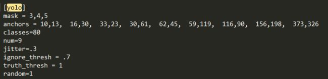
一 、 yolo层参数
二 、 yolo层初始化
需要anchor的加入,除此之外和普通的module没差,所以创建一个DetectionLayer层,其他的功能放到主类Darknet的forward函数里面。
class DetectionLayer(nn.Module):
    def __init__(self, anchors):
        super(DetectionLayer, self).__init__()
        self.anchors = anchors
三、 yolo层的实现
在Darknet类初始化里调用了create_module来构建框架。其中yolo层初始化的过程
        elif x["type"] == "yolo":
            mask = x["mask"].split(",")
            mask = [int(x) for x in mask]

            anchors = x["anchors"].split(",")
            anchors = [int(a) for a in anchors]
            anchors = [(anchors[i], anchors[i+1]) for i in range(0, len(anchors),2)]#mask
            anchors = [anchors[i] for i in mask]

            detection = DetectionLayer(anchors)
            module.add_module("Detection_{}".format(index), detection)
在class Darknet(nn.Module):的forward函数中,主要是predict_transform函数
            elif module_type == 'yolo':
                anchors = self.module_list[i][0].anchors
                #Get the input dimensions
                inp_dim = int (self.net_info["height"])

                #Get the number of classes
                num_classes = int (module["classes"])

                #Transform
                x = x.data
                #将x由 n c w h _> n w*h*3 c
                #batch_size, 3*85, grid_size, grid_size)——》(batch_size, grid_size*grid_size*3, 5+类别数量)
                #在这个过程当中趁机 利用sigmod 将xywh改过来,因为需要xc和sigmod函数,回归嚒

                x = predict_transform(x, inp_dim, anchors, num_classes, CUDA)
                if not write:              #if no collector has been intialised.
                    detections = x
                    write = 1

                else:
                    detections = torch.cat((detections, x), 1)
predict_transform
矩阵思维启蒙
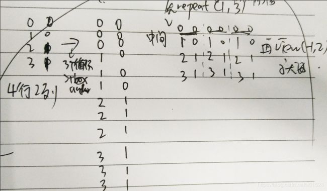
这个用于3个anchors扩展成整个图片的anchors。
torch.repeat()下面这张图,是将4行2列,变成12行2列,首先利用repeat(1,3)行不变列三倍,然后view(-1,2).
np.meshgrid和torch.repeat()
grid = np.arange(grid_size)
a,b = np.meshgrid(grid, grid)
#x_offset即cx,y_offset即cy,表示当前cell左上角坐标
x_offset = torch.FloatTensor(a).view(-1,1) #13*13 其实和上面的图是一样的。
y_offset = torch.FloatTensor(b).view(-1,1)
#一行代表的是一个栅格位置的一个anchor对应的offset,列代表xy的offset值。
#因为是3个anchor,所以行数不变,列数增加为原先3倍,然后再变成2列。
x_y_offset = torch.cat((x_offset, y_offset), 1).repeat(1,num_anchors).view(-1,2).unsqueeze(0)#在第0维度多加1
prediction[:,:,:2] += x_y_offset #bx=sigmoid(tx)+cx,by=sigmoid(ty)+cy
view和transpose共用。再来看下维度变换n,3*85,13,13的输入,如何变成n,13*13*3,85的输出。这样一转换,在第1维度上就可以torch.cat加26*26*3的结果和,52*52*3的结果。表示每一行的每一种anchor对应的85. n,3*85,13,13 _> n,13*13*3,85.
- n,3*85,13,13 _> n,3*85,13*13
prediction = prediction.view(batch_size, bbox_attrs*num_anchors, grid_size*grid_size)
- n,3*85,13*13 _> n,13*13,3*85
prediction = prediction.transpose(1,2).contiguous()
- n,13*13,3*85 _> n,13*13*3,85
prediction = prediction.view(batch_size, grid_size*grid_size*num_anchors, bbox_attrs)
矩阵乘法*
# 这里的anchors本来是一个长度为6的list(三个anchors每个2个坐标),然后在0维上(行)进行了
# grid_size*grid_size个复制,在1维(列)上一次复制(没有变化),即对每个格子都得到三个anchor。
# Unsqueeze(0)的作用是在数组上添加一维,这里是在第0维上添加的。
# 添加grid_size是为了之后的公式bw=pw×e^tw的tw。
# (3,2)_>(13*13*3,2)
anchors = anchors.repeat(grid_size*grid_size, 1).unsqueeze(0)
#对每一个都要对应的乘以相应的anchor
prediction[:,:,2:4] = torch.exp(prediction[:,:,2:4])*anchors# 公式bw=pw×e^tw及bh=ph×e^th,pw为anchorbox的长度
def predict_transform(prediction, inp_dim, anchors, num_classes, CUDA = True):
    """
    prediction表示输出的特征图,(batch_size, 3*85, 13, 13)
     # ——》(batch_size, 13*13*3, 5+80)
    """
    batch_size = prediction.size(0)
    # stride表示的是整个网络的步长
    # 等于图像原始尺寸与yolo层输入的feature mapr尺寸相除
    stride =  inp_dim // prediction.size(2)#416//13=32
    # feature map每条边格子的数量,416//32=13
    grid_size = inp_dim // stride
    # 一个方框属性个数,等于5+类别数量
    bbox_attrs = 5 + num_classes
    # anchors数量
    num_anchors = len(anchors)

    # batch_size, num_anchors * bbox_attrs, grid_size, grid_size  — —》 batch_size, num_anchors*bbox_attrs,, grid_size*grid_size

    prediction = prediction.view(batch_size, bbox_attrs*num_anchors, grid_size*grid_size)

    # batch_size, 85*3, 13*13— —》batch_size, 13*13,3*85
    prediction = prediction.transpose(1,2).contiguous()
    # 将prediction维度转换成(batch_size, grid_size*grid_size*num_anchors, bbox_attrs)。不看batch_size,
    # (grid_size*grid_size*num_anchors, bbox_attrs)相当于将所有anchor按行排列,即一行对应一个anchor属性,此时的属性仍然是feature map得到的值
    prediction = prediction.view(batch_size, grid_size*grid_size*num_anchors, bbox_attrs)
    # 锚点的维度与net块的height和width属性一致。这些属性描述了输入图像的维度,比feature map的规模大(二者之商即是步幅)。因此,我们必须使用stride分割锚点。变换后的anchors是相对于最终的feature map的尺寸
    anchors = [(a[0]/stride, a[1]/stride) for a in anchors]

    #Sigmoid the tX, tY. and object confidencce.tx与ty为预测的坐标偏移值
    prediction[:,:,0] = torch.sigmoid(prediction[:,:,0])
    prediction[:,:,1] = torch.sigmoid(prediction[:,:,1])
    prediction[:,:,4] = torch.sigmoid(prediction[:,:,4])

    #这里生成了每个格子的左上角坐标,生成的坐标为grid x grid的二维数组,a,b分别对应这个二维矩阵的x,y坐标的数组,a,b的维度与grid维度一样。每个grid cell的尺寸均为1,故grid范围是[0,12](假如当前的特征图13*13)
    grid = np.arange(grid_size)
    a,b = np.meshgrid(grid, grid)
    #x_offset即cx,y_offset即cy,表示当前cell左上角坐标
    x_offset = torch.FloatTensor(a).view(-1,1)#13*13
    y_offset = torch.FloatTensor(b).view(-1,1)

    if CUDA:
        x_offset = x_offset.cuda()
        y_offset = y_offset.cuda()
    #一行代表的是一个栅格位置的一个anchor对应的offset,列代表xy的offset值。因为是3个anchor,所以行数不变,列数增加为原先3倍,然后再变成2列。
    x_y_offset = torch.cat((x_offset, y_offset), 1).repeat(1,num_anchors).view(-1,2).unsqueeze(0)#在第0维度多加1

    prediction[:,:,:2] += x_y_offset#bx=sigmoid(tx)+cx,by=sigmoid(ty)+cy

    #[(),(),()]np _> [[],[],[]]tensor,(3,2)
    anchors = torch.FloatTensor(anchors)

    if CUDA:
        anchors = anchors.cuda()
    # 这里的anchors本来是一个长度为6的list(三个anchors每个2个坐标),然后在0维上(行)进行了grid_size*grid_size个复制,在1维(列)上
    # 一次复制(没有变化),即对每个格子都得到三个anchor。Unsqueeze(0)的作用是在数组上添加一维,这里是在第0维上添加的。添加grid_size是为了之后的公式bw=pw×e^tw的tw。
    # (3,2)_>(13*13*3,2)
    anchors = anchors.repeat(grid_size*grid_size, 1).unsqueeze(0)
    #对网络预测得到的矩形框的宽高的偏差值进行指数计算,然后乘以anchors里面对应的宽高(这里的anchors里面的宽高是对应最终的feature map尺寸grid_size),
    # 得到目标的方框的宽高,这里得到的宽高是相对于在feature map的尺寸
    prediction[:,:,2:4] = torch.exp(prediction[:,:,2:4])*anchors#公式bw=pw×e^tw及bh=ph×e^th,pw为anchorbox的长度
    # 这里得到每个anchor中每个类别的得分。将网络预测的每个得分用sigmoid()函数计算得到
    prediction[:,:,5: 5 + num_classes] = torch.sigmoid((prediction[:,:, 5 : 5 + num_classes]))

    prediction[:,:,:4] *= stride#将相对于最终feature map的方框坐标和尺寸映射回输入网络图片(416x416),即将方框的坐标乘以网络的stride即可

    return prediction