Back Ground
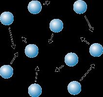
A random walk is a mathematical object which describes a path that consists of a succession of random steps. For example, the path traced by a molecule as it travels in a liquid or a gas, the search path of a foraging animal, superstring behavior, the price of a fluctuating stock and the financial status of a gambler can all be approximated by random walk models, even though they may not be truly random in reality.
The term random walk was first introduced by Karl Pearson in 1905.
Abstract
- Random Walks
- Random Walks and Diffusion
The Main Body
What is Random Walk
The simplest random walk to understand is a 1-dimensional walk. Suppose that the black dot below is sitting on a number line. The black dot starts in the center.
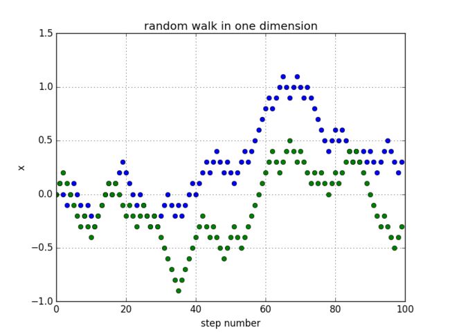
Then, it takes a step, either forward or backward, with equal probability. It keeps taking steps either forward or backward each time. Let's call the 1st step a1, the second step a2, the third step a3 and so on. Each "a" is either equal to +1 (if the step is forward) or -1 (if the step is backward). The picture below shows a black dot that has taken 5 steps and ended up at -1 on the number line.
code:
import random
import matplotlib.pyplot as plt
class random_walks:
    def __init__(self,n=100,step_length=0.1):
        self.x=[0]
        self.y=[0]
        self.x2=[0]
        self.n=n
        self.l=step_length
    def walk1(self):#random walk with step_length=1
        for i in range(1,self.n):
            self.x.append(i)
            temp=random.random()
            if temp < 0.5:
                self.y.append(self.y[-1]-self.l)
            elif temp > 0.5:
                self.y.append(self.y[-1]+self.l)
            self.x2.append(self.x2[-1]+self.l**2)
    def walk2(self):#random walk with random step-length
        for i in range(1,self.n):
            self.x.append(i)
            temp=random.random()
            self.l=random.random()
            if temp < 0.5:
                self.y.append(self.y[-1]-self.l)
            elif temp > 0.5:
                self.y.append(self.y[-1]+self.l)
            self.x2.append(self.x2[-1]+self.l**2)
    def show1(self):
        plt.plot(self.x,self.y,'o')
        plt.title('random walk in one dimension')
        plt.xlabel('step number')
        plt.ylabel('x')
        plt.grid(True)
    def show2(self):
        plt.plot(self.x,self.x2,'.',label='$$ versus time')
        plt.title('random walk in one dimension')
        plt.xlabel('step number')
        plt.ylabel('$$')
        plt.legend(frameon=True)
        plt.grid(True)
a=random_walks()
a.walk1()
a.show1()
b=random_walks()
b.walk1()
b.show1()
-
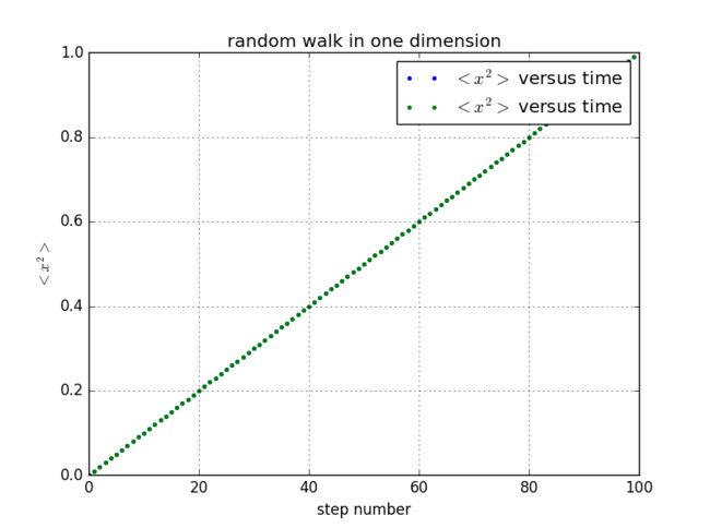
random walk with step length=1:
-
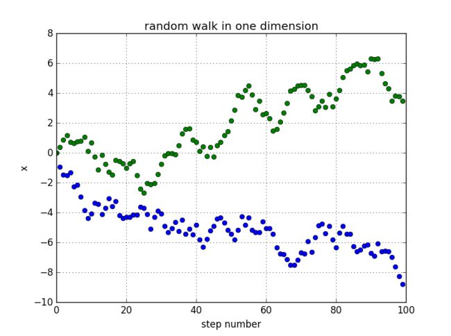
random walk with random step lengths:
Random Walks and Diffusion
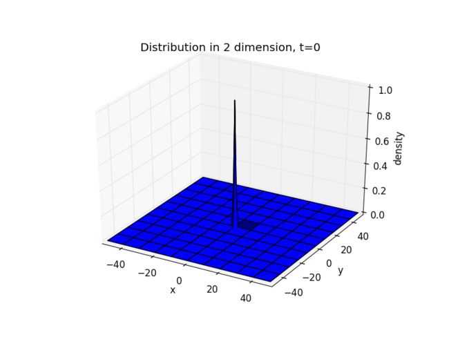
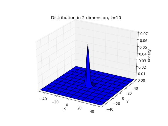
An alternative way to describe the same physics involves the density of particles, ρ(x,y,z,t), which can be conveniently defined if the system contains a large number of particles (walkers). The idea, known as coarse graining, is to consider regions of space that are big enough to contain a large number of particles so that the density ( =mass/ volume) can be meaningfully defined. The density is then proportional to the probability per unit volume per unit time, denoted by P(x,y,z, t), to find a particle at (x, y, z) at time t. Thus, ρ and P obey the same equation.
To find this equation, we focus back on an individual random walker. We assume that it is confined to take steps on a simple-cubic lattice, and that it makes one "walking step" each time step. P(i, j, k, n) is the probability to find the particle at the side (i, j, k) at time n. Since we are on a simple cubic lattice, there are 6 different nearest neighbor sites. If the walker is on one of these sites at time n-1, there is a probability of 1/6 that it will then move to site (i, j, k) at time n. Hence, the total probability to arrive at (i, j, k) is :
Rearranging the equation,and it suggests takking the continuum limit,which lead to:
This derivation shows the close connection between the random walks and diffusion.The density ρ obeys the same equation:
For ease of notation we will assume that ρ is a function of only one spatial dimension, x, although everything we do below can readily be extended to two or three dimensions. We can then write
so that the first index corresponds to space and the second to time.
and the finite-difference version of this is
rearranging to express the density at time step n+1 in terms of ρ at step n we find
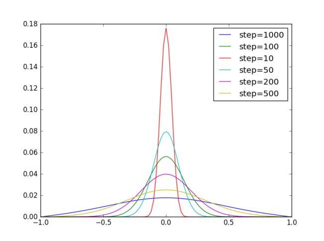
code:
import pylab as plt
import numpy as np

N=101
dx=2./(N-1)
dt=0.1
D=1./4*(dx**2)/dt

class diffusion:
    def __init__(self,step):
        self.step=step
        self.x=np.linspace(-1,1,N)
        self.y=np.linspace(0,0,N)
        self.old_y=np.linspace(0,0,N)
        self.y[50]=1

    def update(self):
        for i in range(N):
            self.old_y[i]=self.y[i]

        for i in range(1,N-1):
            self.y[i]=self.old_y[i]+D*dt/(dx**2)*(self.old_y[i+1]+self.old_y[i-1]-2*self.old_y[i])

    def fire(self):
        for i in range(self.step):
            self.update()
            i+=1

        plt.plot(self.x,self.y,label="step="+str(self.step))


A=diffusion(1000)
A.fire()
A=diffusion(100)
A.fire()
A=diffusion(10)
A.fire()
A=diffusion(50)
A.fire()
A=diffusion(200)
A.fire()
A=diffusion(500)
A.fire()
plt.legend(loc="best")
plt.show()
import matplotlib.pyplot as plt
import numpy as np
import random
class rand_walks:
    def __init__(self,l=100,N=5000,time=1000):
        self.l=l
        self.N=N
        self.n=time
        self.loca=[[0]*self.l]
    def walk(self):
        self.loca[-1][int(self.l/2)]=self.N
        counter=0
        while(1):
            counter+=1
            temp=[0]*self.l
            for  i in range(self.l-2):
                for j in range(self.loca[-1][i+1]):
                    rand=random.random()
                    if rand>0.5:
                        temp[i+2]+=1
                    elif rand<0.5:
                        temp[i]+=1
            self.loca.append(temp)
            if counter>self.n:
                break
    def show(self):
        x=np.arange(0,100,1)
        plt.plot(x,self.loca[-1],'.')
        plt.plot(x,self.loca[-1],label='time=%.f'%self.n)
        plt.title('random walks of %.f particles'%self.N)
        plt.xlabel('x')
        plt.ylabel('number of particles')
        plt.grid(True)
        plt.legend(frameon=True)

b=rand_walks(time=10)
b.walk()
b.show()
b=rand_walks(time=100)
b.walk()
b.show()
b=rand_walks(time=1000)
b.walk()
b.show()
Acknowledgement
Nicholas J.Giodano's computational physics.
