Exercise 13：Frequency Spectrum of Waves on a String

Background

In physics, a wave is an oscillation accompanied by a transfer of energy that travels through a medium (space or mass). Frequency refers to the addition of time. Wave motion transfers energy from one point to another, which displace particles of the transmission medium–that is, with little or no associated mass transport. Waves consist, instead, of oscillations or vibrations (of a physical quantity), around almost fixed locations.

Abstract

This article is about using numerical method to solve wave function, especially for a wave spreading in a string. Further more, it will discuss the semirealistic case and realistic case,just like piano strings, with which whether we considering friction.

The Main Body

6.12: Gaussian initial string displacements are convenient for the calculations of this section, but are not very realistic. When a real string, such as a guitar string, is plucked, the initial string displacement is more accurately described by two straight lines that start at the ends of the string (we assume fixed ends) and end at the excitation point, as illustrated in Figure 6.4. Compare the power spectrum for a string excited in this manner with results found above for a Gaussian initial wavepacket.

Wave Equation

In order to solve this equation it must give the boundary condition.We suppose that each ends of the string is well-fixed.To construct a numerical approach to the wave equation we treat both x and t as discrete variables.Derive the needed expression for the second partial derivative, and inserting it into the wave equation, we obtain：

To write the the expression at next time step the result from above can be written as：

Where r=1 is commanded.

code：

import numpy as np

import matplotlib.pyplot

from pylab import *

from math import *

import mpl_toolkits.mplot3d

def power_spe(xe,xo):#xe excited, xo observed

dx=0.01

c=300.0 #speed

dt=dx/c

length=int(1.0/dx)

time=3000

k=1000

y=[[0 for i in range(length)]for n in range(time)]#i represents x, n represents t

#initialize

for i in range(length):

y[0][i]=exp(-k*(i*dx-xe)**2)

y[1][i]=exp(-k*(i*dx-xe)**2)

r=c*dt/dx

#iteration

for n in range(time-2):

for i in range(1,length-1):

y[n+2][i]=2*(1-r**2)*y[n+1][i]-y[n][i]+r**2*(y[n+1][i+1]+y[n+1][i-1])

y=array(y)

yo=[]

t=array(range(time))*dt

for n in range(time):

yo.append(y[n][int(xo/dx)])

p=abs(np.fft.rfft(yo))**2

f = np.linspace(0, int(1/dt/2), len(p))

plot(f, p)

xlim(0,3000)

xlabel('Frequency(Hz)')

ylabel('Power')

title('Power spectrum')

text(2000,12000,'$x_{observed}=$'+str(xo))

figure(figsize=[16,16])

subplot(221)

power_spe(0.8,0.05)

subplot(222)

power_spe(0.8,0.1)

subplot(223)

power_spe(0.8,0.4)

subplot(224)

power_spe(0.8,0.5)

show()

Conclusion

First of all , if we choose triangular wave as initial wave

We can see there are several peaks in the power spectrum, with the increasing of frequency, the peakvalue get smaller.
Then we change the excited point. If the string is excited from x = 0.3, the signal is:

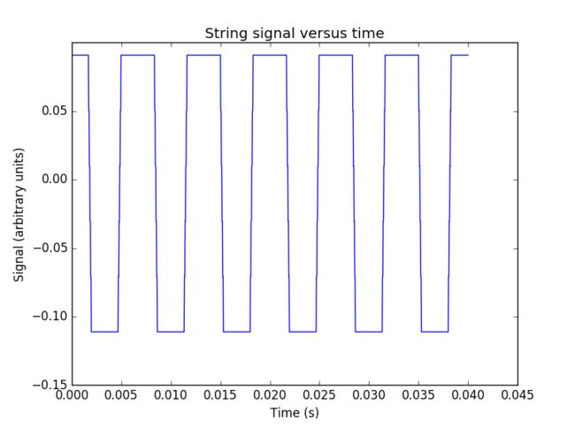
The number of peak has increased.

problem 6.13:

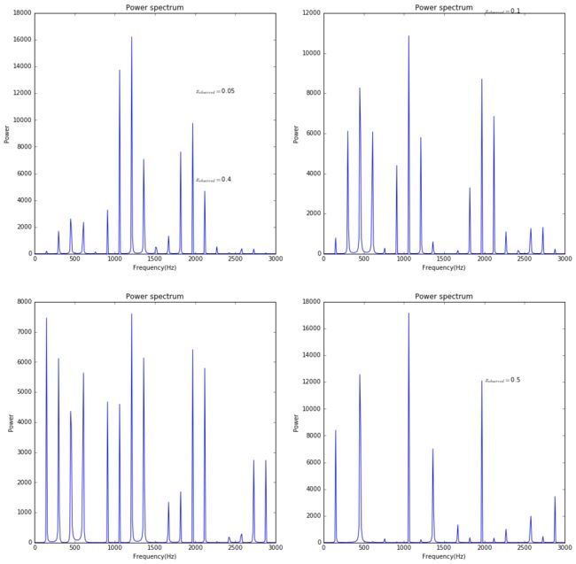
Consider the power spectra for waves on a string as a function of where the string vibration is observed,x0.

code:

import numpy as np

import matplotlib.pyplot

from pylab import *

from math import *

import mpl_toolkits.mplot3d

def power_spe(xe,xo):#xe excited, xo observed

dx=0.01

c=300.0 #speed

dt=dx/c

length=int(1.0/dx)

time=3000

k=1000

y=[[0 for i in range(length)]for n in range(time)]#i represents x, n represents t

#initialize

for i in range(length):

y[0][i]=exp(-k*(i*dx-xe)**2)

y[1][i]=exp(-k*(i*dx-xe)**2)

r=c*dt/dx

#iteration

for n in range(time-2):

for i in range(1,length-1):

y[n+2][i]=2*(1-r**2)*y[n+1][i]-y[n][i]+r**2*(y[n+1][i+1]+y[n+1][i-1])

y=array(y)

yo=[]

t=array(range(time))*dt

for n in range(time):

yo.append(y[n][int(xo/dx)])

p=abs(np.fft.rfft(yo))**2

f = np.linspace(0, int(1/dt/2), len(p))

plot(f, p)

xlim(0,3000)

xlabel('Frequency(Hz)')

ylabel('Power')

title('Power spectrum')

text(2000,12000,'$x_{observed}=$'+str(xo))

figure(figsize=[16,16])

subplot(221)

power_spe(0.8,0.05)

subplot(222)

power_spe(0.8,0.1)

subplot(223)

power_spe(0.8,0.4)

subplot(224)

power_spe(0.8,0.5)

show()

Conclusion

First of all, if the string is excited at 50% of string (Gaussian profile), the power spectra at different nodes are:

Then, if the string is excited at 60% of string , the power spectra at different nodes are:

Last, if the string is excited at 80% of string , the power spectra at different nodes are: