TensorFlow学习笔记(5) 卷积神经网络

目录

 

卷积神经网络的基本结构

卷积层

池化层

经典卷积网络

LeNet-5模型

Inception-v3模型

迁移学习

---

卷积神经网络的基本结构

前面所提到的MNIST是一个相对简单的数据集，而在其他更复杂的图像识别数据集上，卷积神经网络有更好的表现。比如Cifar数据集和ImageNet数据集。Cifar分为Cifar-10和Cifar-100两个问题，都是32*32的彩色图片，Cifar-10问题收集了来自10个不同种类的60000张图片。而ImageNet数据集中的分辨率更高，图像也更加复杂。

在之前所提到的神经网络每两层之间的所有结点都是有边相连的，所以成为全连接神经网络，这种网络的最大问题是参数数量过大。而卷积神经网络与之相比有所差异，相邻两层之间只有部分节点相连，为了展示每一层神经元的维度，一般会将每一层卷积层的节点组织成一个三维矩阵。两种神经网络的训练流程没有任何区别，唯一的区别就在于神经网络中相邻两层的链接方式。

一个卷积网络具体由以下五种结构组成：

• 输入层：输入层一般代表了一个图片的三维矩阵，其中长和宽代表了图像的大小，深度代表了图像的彩色通道。比如黑白图片的深度为1，RGB彩色图片的深度为三。在神经网络种，每一层的三维矩阵都会转化为下一层的三维矩阵，直到最后的全连接层。
• 卷积层：卷积层中每一个节点的输入只是上一层神经网络的小块，常用的大小有5*5或3*3。卷积层试图将神经网络种每一小块进行更加深入的剖析。一般来说，经过卷积层处理过的节点矩阵会变得更深。
• 池化层：该层不会改变三维矩阵的深度，但会缩小矩阵的大小，达到减少整个神经网络的参数的目的。
• 全连接层：卷积神经网络最后一般会是由1到2个全连接层来给出最后的分类结果，通过卷积层和池化层对图像特征的提取，利用全连接层实现对图像的分分类。
• Softmax层：主要用于分类问题，通过该层可以得到当前样例属于不同种类的概率分布。

卷积层

卷积层中最重要的部分成为过滤器或者内核，可以将当前神经网络上的一个子节点矩阵转化为下一层神经网络上的一个单位节点矩阵（长宽为1，深度不限）。过滤器的尺寸一般为3*3或5*5，需要人工指定，成为过滤器尺寸；处理得到的单位节点的深度也需要人工指定，称为为过滤器的深度。在卷积神经网络中，每一个卷积层中使用的过滤器的参数都是一样的。

经过卷积操作的图像一般大小变为：out = (in - kernel_size +1)/stride

在TF中可以实现一个卷积层的前向传播：

import tensorflow as tf

#创建过滤器的权重变量和偏置项变量
#卷积层的参数个数只与过滤器的尺寸、深度以及当前层节点矩阵的深度有关，因此声明的参数变量为四维矩阵
#前两个维度代表了过滤器尺寸，第三个代表当前层的深度，第四个代表过滤器的深度
filter_weight = tf.get_variable('weights', [5, 3, 3, 16], initializar=tf.truncated_normal_initializer(stddev=0.1))
biases = tf.get_variable('biases', [16], initializer=tf.constant_initializer(0.1))

#tf.nn.conv2d可以实现卷积层前向传播的算法
#该函数第一个输入为当前层的节点矩阵，该矩阵为四维矩阵，第一个参数代表第n个图片，后三个代表一个节点矩阵
#第二个输入代表卷积层的权重
#第三个输入为不同维度上的步长从，该矩阵为四维矩阵，但第一个和第四个参数一定为1，中间两个代表在长和宽上的步长
#第四个输入为填充padding的方法，其中SAME表示全0填充，VALID表示不填充
conv = tf.nn.conv2d(input, filter_weight, strides=[1,1,1,1], padding='SAME')

#给每一个节点加上偏置项
bias = tf.nn.bias_add(conv, biases)

#通过激活函数去线性化
actived_conv = tf.nn.relu(bias)

池化层

池化层可以非常有效的缩短矩阵的尺寸，从而减少最后全连接层中的参数。使用池化层可以加快计算速度也有防止过拟合问题的作用。池化层过滤器的计算不是节点的加权和，而是采用更加简单的最大值或者平均值运算，称之为最大池化层或者平均池化层。池化层与卷积层过滤器参数的设置移动的方式都是一样的。池化层过滤器除了在长和宽两个维度移动之外，它还需要再深度这个维度移动。

下面的TF程序实现了最大池化层的前向传播算法：

#tf.nn.max_pool可以实现最大池化层的前向传播的算法
#该函数第一个输入为卷积层得到的结果
#第二个输入代表过滤器的尺寸ksize，该矩阵为四维矩阵，但第一个和第四个参数一定为1，中间两个代表过滤器的长和宽
#第三个输入为不同维度上的步长从，该矩阵为四维矩阵，但第一个和第四个参数一定为1，中间两个代表在长和宽上的步长
#第四个输入为填充padding的方法，其中SAME表示全0填充，VALID表示不填充
pool = tf.nn.max_pool(actived_conv, ksize=[1, 3, 3, 1], strides=[1,2,2,1], padding='SAME')

#平均池化层
pool = tf.nn.avg_pool(actived_conv, ksize=[1, 3, 3, 1], strides=[1,2,2,1], padding='SAME')

经典卷积网络

LeNet-5模型

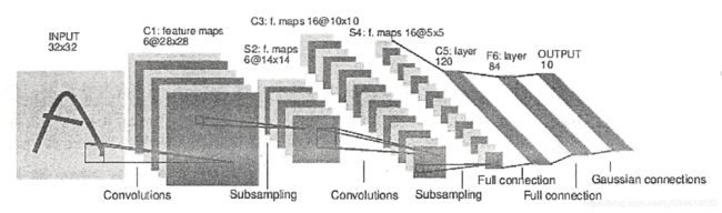
LeNet-5模型一共有7层：

1. 卷积层。这一层的输入是原始图像像素，模型接受的输入层大小为32*32*1。过滤器尺寸为5*5，深度为6，不使用全0填充，步长为1。输出尺寸为32-5+1=28，深度为6。该卷积层共有5*5*1*6+6=156个参数。
2. 池化层。这一层的输入是第一层的输出，是一个28*28*6的节点矩阵。本层过滤器尺寸为2*2，长和宽步长为2，输出矩阵为14*14*6。
3. 卷积层。本层输入矩阵尺寸大小为14*14*6。使用过滤器大小为5*5*16，不使用全0填充，步长为1。输出矩阵大小为10*10*16，共有5*5*6*16+16=2416个参数。
4. 池化层。输入矩阵10*10*16，过滤器大小2*2，步长2，输出5*5*16。
5. 全连接层。输入矩阵5*5*16，过滤器大小5*5，输出长度为120的向量，共有5*5*16*120+120=48120个参数
6. 全连接层。输入节点120，输出节点84，总参数120*84+84=10164个。
7. 全连接层。输入节点84，输出节点10，总参数120*84+84=10164个。

下面为一个TF程序实现类似该模型的卷积神经网络解决MNIST数字识别问题：

• mnist_cnn_inference.py

import tensorflow as tf

#定义神经网络结构相关的参数
INPUT_NODE = 784
OUTPUT_NODE = 10

IMAGE_SIZE = 28
NUM_CHANNELS = 1
NUM_LABELS = 10

#第一层卷积层滤波器的尺寸和深度
CONV1_DEEP = 32
CONV1_SIZE = 5
#第二层卷积层滤波器的尺寸和深度
CONV2_DEEP = 64
CONV2_SIZE = 5
#全连接层的节点个数
FC_SIZE = 512

#定义卷积神经网络，train用于区分训练过程和测试过程
def inference(input_tensor, train, regularizer):
    #声明第一层卷积层，输入28*28*1，输出28*28*32
    with tf.variable_scope('layer1-conv1'):
        conv1_weights = tf.get_variable('weight', [CONV1_SIZE, CONV1_SIZE, NUM_CHANNELS, CONV1_DEEP],
                                        initializer=tf.truncated_normal_initializer(stddev=0.1))
        conv1_biases = tf.get_variable('bias', [CONV1_DEEP], initializer=tf.constant_initializer(0.0))
        conv1 = tf.nn.conv2d(input_tensor, conv1_weights, strides=[1, 1, 1, 1], padding='SAME')
        conv1 = tf.nn.relu(tf.nn.bias_add(conv1, conv1_biases))

    #声明第一层池化层，输入28*28*32，输出14*14*32
    with tf.variable_scope('layer2-pool1'):
        pool1 = tf.nn.max_pool(conv1, ksize=[1, 2, 2, 1], strides=[1, 2, 2, 1], padding='SAME')

    #声明第三层卷积层，输入14*14*32，输出14*14*64
    with tf.variable_scope('layer3-conv2'):
        conv2_weights = tf.get_variable('weight', [CONV2_SIZE, CONV2_SIZE, CONV1_DEEP, CONV2_DEEP],
                                        initializer=tf.truncated_normal_initializer(stddev=0.1))
        conv2_biases = tf.get_variable('bias', [CONV2_DEEP], initializer=tf.constant_initializer(0.0))
        conv2 = tf.nn.conv2d(pool1, conv2_weights, strides=[1, 1, 1, 1], padding='SAME')
        conv2 = tf.nn.relu(tf.nn.bias_add(conv2, conv2_biases))

    #声明第四层池化层，输入14*14*64，输出7*7*64
    with tf.variable_scope('layer4-pool2'):
        pool2 = tf.nn.max_pool(conv2, ksize=[1, 2, 2, 1], strides=[1, 2, 2, 1], padding='SAME')

    #将第四层输出格式（7*7*64)转化为第五层的输入格式一个向量
    pool2_shape = pool2.get_shape().as_list()
    nodes = pool2_shape[1] * pool2_shape[2] * pool2_shape[3]   #7*7*64,pool2_shape[0]为一个bantch中数据的个数
    reshaped = tf.reshape(pool2, [pool2_shape[0], nodes])

    #声明第五层全连接层，输入7*7*64=3136长度的向量，输出512
    #引入dropout概念，会在训练时随机将部分节点的输出改为0，避免过拟合问题，一般用在全连接层
    with tf.variable_scope('layer5-fc1'):
        fc1_weights = tf.get_variable('weight', [nodes, FC_SIZE],
                                      initializer=tf.truncated_normal_initializer(stddev=0.1))
        fc1_biases = tf.get_variable('bias', [FC_SIZE], initializer=tf.constant_initializer(0.1))
        if regularizer != None:#只有全连接层的权重需要加入正则化
            tf.add_to_collection('losses', regularizer(fc1_weights))
        fc1 = tf.nn.relu(tf.matmul(reshaped, fc1_weights) + fc1_biases)
        if train:fc1 = tf.nn.dropout(fc1, 0.5)

    #声明第6层全连接层，输入512，输出10，通过softmax之后得到最后的分类结果
    with tf.variable_scope('layer6-fc2'):
        fc2_weights = tf.get_variable('weight', [FC_SIZE, NUM_LABELS],
                                      initializer=tf.truncated_normal_initializer(stddev=0.1))
        fc2_biases = tf.get_variable('bias', [NUM_LABELS], initializer=tf.constant_initializer(0.1))
        if regularizer != None:#只有全连接层的权重需要加入正则化
            tf.add_to_collection('losses', regularizer(fc2_weights))
        fc2 = tf.matmul(fc1, fc2_weights) + fc2_biases

    return fc2

• mnist_cnn_train.py

import os
import tensorflow as tf
from tensorflow.examples.tutorials.mnist import input_data
import mnist_cnn_inference
import numpy as np


# 配置神经网络的参数
BATCH_SIZE = 100
LEARNING_RATE_BASE = 0.001
LEARNING_RATE_DECAY = 0.99
REGULARIZATION_RATE = 0.0001 #描述模型复杂度的正则化项在损失函数中的系数
TRAINING_STEPS = 10000
MOVING_AVERAGE_DECAY = 0.99 #滑动平均衰减率

#模型保存的路径和文件名
MODEL_SAVE_PATH = '/mnist_cnn_model/'
MODEL_SAVE_NAME = 'mnist_cnn_model.ckpt'

def train(mnist):
    x = tf.placeholder(tf.float32, [BATCH_SIZE, mnist_cnn_inference.IMAGE_SIZE, mnist_cnn_inference.IMAGE_SIZE,
                                    mnist_cnn_inference.NUM_CHANNELS], name='x-input')
    y_ = tf.placeholder(tf.float32, [None, mnist_cnn_inference.OUTPUT_NODE], name='y-input')
    regularizer = tf.contrib.layers.l2_regularizer(REGULARIZATION_RATE)

    #直接使用mnist_cnn_inference.py中定义的前向传播结果
    y = mnist_cnn_inference.inference(x, train=False, regularizer=regularizer)
    global_step = tf.Variable(0, trainable=False)

    # 生成一个滑动平均的类，并在所有变量上使用滑动平均
    variables_averages = tf.train.ExponentialMovingAverage(MOVING_AVERAGE_DECAY, global_step)
    variables_averages_op = variables_averages.apply(tf.trainable_variables())

    # 计算交叉熵及当前batch中的所有样例的交叉熵平均值,并求出损失函数
    cross_entropy = tf.nn.sparse_softmax_cross_entropy_with_logits(logits=y, labels=tf.argmax(y_, 1))
    cross_entropy_mean = tf.reduce_mean(cross_entropy)
    loss = cross_entropy_mean + tf.add_n(tf.get_collection('losses'))

    # 定义指数衰减式的学习率以及训练过程
    learning_rate = tf.train.exponential_decay(LEARNING_RATE_BASE, global_step, mnist.train.num_examples / BATCH_SIZE, LEARNING_RATE_DECAY)
    train_step = tf.train.GradientDescentOptimizer(learning_rate).minimize(loss, global_step=global_step)
    with tf.control_dependencies([train_step, variables_averages_op]):
        train_op = tf.no_op(name='train')

    #初始化TF持久化类
    saver = tf.train.Saver()

    with tf.Session() as sess:
        sess.run(tf.global_variables_initializer())

        for i in range(TRAINING_STEPS):
            xs, ys = mnist.train.next_batch(BATCH_SIZE)
            reshaped_xs = np.reshape(xs, [BATCH_SIZE, mnist_cnn_inference.IMAGE_SIZE, mnist_cnn_inference.IMAGE_SIZE,
                                    mnist_cnn_inference.NUM_CHANNELS])
            _, loss_value, step = sess.run([train_op, loss, global_step], feed_dict={x: reshaped_xs, y_: ys})
            # if i%500 == 0:
            print('After %d training steps, loss on training batch is %g' % (step, loss_value))
            saver.save(sess, os.path.join(MODEL_SAVE_PATH, MODEL_SAVE_NAME), global_step=global_step)

def main(argv=None):
    mnist = input_data.read_data_sets("MNIST_data", one_hot=True)
    train(mnist)

if __name__ =='__main__':
    tf.app.run()

如何设计卷积神经网络的架构？下面的正则表达式总结了一些经典的用于图片分类问题的卷积神经网络架构：

输入层>>（卷积层+ >> 池化层？） >> 全连接层+

在上面的公式中【+表示一个或多个】，【？表示一个或没有】。一般的卷积神经网络都满足这个结构。在过滤器的深度上，一般卷积网络都采取逐层递增的方式。

Inception-v3模型

Inception结构是一种和上一个模型结构完全不同的卷积神经网络。在LeNet-5中，不同卷积层通过串联的方式连接在一起，而Inception结构是将不同的卷积层通过并联的方式结合在一起。

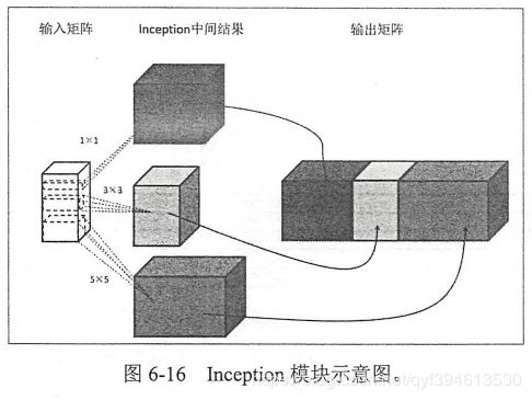
Inception模块会首先使用不同尺寸的过滤器处理输入矩阵，不同的矩阵代表Inception模块的一条计算路径。虽然过滤器的大小不一，但如果所有的过滤器都是用全0填充且步长为1，那么得到的矩阵的长与宽都与输入矩阵一致。最后将不同过滤器处理的结果矩阵拼接成更深的矩阵。

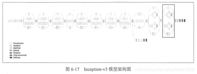
如上图所示，Inception-v3模型一共有46层，由11个Inception模块组成，其中方框中为一个Inception模块，共有96个卷积层。由TensorFlow-Slim工具可以更加简洁的实现一个卷积层，从而更好的实现复杂的卷积神经网络。

TensorFlow-Slim是tensorflow中一个高级api，可以更快速简洁的实现卷积操作。

#使用TF原始API实现卷积层
with tf.variable_scope('layer1-conv1'):
    conv1_weights = tf.get_variable('weight', [1,1,1,1], initializer=tf.truncated_normal_initializer(stddev=0.1))
    conv1_biases = tf.get_variable('bias', [2], initializer=tf.constant_initializer(0.0))
    conv1 = tf.nn.conv2d(input, conv1_weights, strides=[1, 1, 1, 1], padding='SAME')
    conv1 = tf.nn.relu(tf.nn.bias_add(conv1, conv1_biases))
    
    
#使用TensorFlow-Slim实现卷积层
#其中有三个参数必填：输入节点矩阵，卷积过滤器的深度，卷积过滤器的长和宽
#可选参数：过滤器移动步长、是否使用全0填充，激活函数的选择、变量的命名空间
net = slim.conv2d(input, 32, [3,3])

下面为Inception-v3模型中的Inception模块的实现

import tensorflow as tf

#slim.arg_scope函数用于设置默认参数取值
#slim.arg_scope第一个参数是一个函数列表，这些函数都会使用后面的默认参数
with slim.arg_scope([slim.conv2d, slim.max_pool2d, slim.avg_pool2d], stride=1, padding='SAME'):
    net = 上一层的输出
    #整个模块声明的命名空间
    with tf.variable_scope('Mixed_7c'):
        #为该模块每一条路径声明一个命名空间
        with tf.variable_scope('Branch_0'):
            branch_0 = slim.conv2d(net, 320, [1, 1], scope='Conv2d_0a_1x1')
        with tf.variable_scope('Branch_1'):
            branch_1 = slim.conv2d(net, 384, [1, 1], scope='Conv2d_0a_1x1')
            #tf.contact可以将多个矩阵拼接起来,第一个参数3表示矩阵在深度上进行拼接
            branch_1 = tf.concat(3,
                                 [slim.conv2d(branch_1, 384, [1, 3], scope='Conv2d_0b_1x3'),
                                  slim.conv2d(branch_1, 384, [3, 1], scope='Conv2d_0c_3x1')])

        with tf.variable_scope('Branch_2'):
            branch_2 = slim.conv2d(net, 448, [1, 1], scope='Conv2d_0a_1x1')
            branch_2 = slim.conv2d(branch_2, 384, [3, 3], scope='Conv2d_0b_3x3')
            branch_2 = tf.concat(3,
                                 [slim.conv2d(branch_2, 384, [1, 3], scope='Conv2d_0c_1x3'),
                                  slim.conv2d(branch_2, 384, [3, 1], scope='Conv2d_0d_3x1')])
        with tf.variable_scope('Branch_3'):
            branch_3 = slim.avg_pool2d(net, [3, 3], scope='AvgPool_0a_3x3')
            branch_3 = slim.conv2d(branch_3, 192, [1, 1], scope='Conv2d_0b_1x1')

        net = tf.concat(3, [branch_0, branch_1, branch_2, branch_3])

迁移学习

迁移学习，就是将一个问题上训练好的模型通过简单的调整使其适用于一个新的问题，比如保留训练好的Inception-v3中的所有参数，只替换最后一层全连接层。可以将前面的层理解为一个图像特征的提取器，通过将特征向量作为输入得到一个新的全连接层来解决新的分类问题。

当数据量足够时，迁移学习的效果不如重新训练，但是在数据不够或运算能力不足时，就很有用。

• 首先定义一些读取数据的函数：

import glob
import os.path
import random
import numpy as np
import tensorflow as tf
from tensorflow.python.platform import gfile

# 模型和样本路径的设置
# inception-v3模型瓶颈层的节点数
BOTTLENECK_TENSOR_SIZE = 2048

# inception-v3模型中代表瓶颈层结果的张量名称，谷歌提供的inception-v3模型中，这个张量名称就是'pool_3/_reshape:0'
# 训练过程中，可以利用tensor.name来获取张量的名称
BOTTLENECK_TENSOR_NAME = 'pool_3/_reshape:0'

# 图像输入张量所对应的名称
JPEG_DATA_TENSOR_NAME = 'DecodeJpeg/contents:0'

# 保存的模型文件目录
MODEL_DIR = '../../datasets/inception_dec_2015'
# 下载的谷歌训练好的inception-v3模型文件名
MODEL_FILE= 'tensorflow_inception_graph.pb'

# 因为一个训练数据会被使用多次，所以可以将原始图像通过inception-v3模型计算得到的特征向量保存在文件中，
# 以免重复计算，下面是这些文件的存放地址。
CACHE_DIR = '../../datasets/bottleneck'

# 图片数据文件夹
# 该文件夹中每一个子文件夹代表一个需要区分的类别，每个子文件夹中存放了对应类别的图片
INPUT_DATA = '../../datasets/flower_photos'

# 验证集百分比
VALIDATION_PERCENTAGE = 10
# 测试集百分比
TEST_PERCENTAGE = 10

LEARNING_RATE = 0.01
STEPS = 4000
BATCH = 100

# 把样本中所有的图片列表并按训练、验证、测试数据分开
def create_image_lists(testing_percentage, validation_percentage):
    # 定义一个result字典，key存储类别名称， 与key对应的value也是一个字典，存储所有该类的图片名称
    result = {}
    # 获取当前目录下所有的子目录
    sub_dirs = [x[0] for x in os.walk(INPUT_DATA)]
    is_root_dir = True
    for sub_dir in sub_dirs:
        if is_root_dir:
            is_root_dir = False
            continue

        extensions = ['jpg', 'jpeg', 'JPG', 'JPEG']

        file_list = []
        dir_name = os.path.basename(sub_dir)
        for extension in extensions:
            file_glob = os.path.join(INPUT_DATA, dir_name, '*.' + extension)
            file_list.extend(glob.glob(file_glob))
        if not file_list: continue

        label_name = dir_name.lower()

        
        training_images = []
        testing_images = []
        validation_images = []
        for file_name in file_list:
            base_name = os.path.basename(file_name)

            # 随机划分数据
            chance = np.random.randint(100)
            if chance < validation_percentage:
                validation_images.append(base_name)
            elif chance < (testing_percentage + validation_percentage):
                testing_images.append(base_name)
            else:
                training_images.append(base_name)

        result[label_name] = {
            'dir': dir_name,
            'training': training_images,
            'testing': testing_images,
            'validation': validation_images,
        }
    return result

# 通过类别名称、所属数据集和图片编号获取一张图片的地址
def get_image_path(image_lists, image_dir, label_name, index, category):
    label_lists = image_lists[label_name]
    category_list = label_lists[category]
    mod_index = index % len(category_list)
    base_name = category_list[mod_index]
    sub_dir = label_lists['dir']
    full_path = os.path.join(image_dir, sub_dir, base_name)
    return full_path

# 获取Inception-v3模型处理之后的特征向量的文件地址
def get_bottleneck_path(image_lists, label_name, index, category):
    return get_image_path(image_lists, CACHE_DIR, label_name, index, category) + '.txt'

# 使用加载的训练好的Inception-v3模型处理一张图片，得到这个图片的特征向量
def run_bottleneck_on_image(sess, image_data, image_data_tensor, bottleneck_tensor):

    bottleneck_values = sess.run(bottleneck_tensor, {image_data_tensor: image_data})
    # 将四维数组压缩为一个特征向量
    bottleneck_values = np.squeeze(bottleneck_values)
    return bottleneck_values

# 先试图寻找已经计算且保存下来的特征向量，如果找不到则先计算这个特征向量，然后保存到文件
def get_or_create_bottleneck(sess, image_lists, label_name, index, category, jpeg_data_tensor, bottleneck_tensor):
    label_lists = image_lists[label_name]
    sub_dir = label_lists['dir']
    sub_dir_path = os.path.join(CACHE_DIR, sub_dir)
    if not os.path.exists(sub_dir_path): os.makedirs(sub_dir_path)
    bottleneck_path = get_bottleneck_path(image_lists, label_name, index, category)
    if not os.path.exists(bottleneck_path):

        image_path = get_image_path(image_lists, INPUT_DATA, label_name, index, category)

        image_data = gfile.FastGFile(image_path, 'rb').read()

        bottleneck_values = run_bottleneck_on_image(sess, image_data, jpeg_data_tensor, bottleneck_tensor)

        bottleneck_string = ','.join(str(x) for x in bottleneck_values)
        with open(bottleneck_path, 'w') as bottleneck_file:
            bottleneck_file.write(bottleneck_string)
    else:

        with open(bottleneck_path, 'r') as bottleneck_file:
            bottleneck_string = bottleneck_file.read()
        bottleneck_values = [float(x) for x in bottleneck_string.split(',')]

    return bottleneck_values

# 随机获取一个batch的图片作为训练数据，并求出他的瓶颈层tensor
def get_random_cached_bottlenecks(sess, n_classes, image_lists, how_many, category, jpeg_data_tensor, bottleneck_tensor):
    bottlenecks = []
    ground_truths = []
    for _ in range(how_many):
        label_index = random.randrange(n_classes)
        label_name = list(image_lists.keys())[label_index]
        image_index = random.randrange(65536)
        bottleneck = get_or_create_bottleneck(
            sess, image_lists, label_name, image_index, category, jpeg_data_tensor, bottleneck_tensor)
        ground_truth = np.zeros(n_classes, dtype=np.float32)
        ground_truth[label_index] = 1.0
        bottlenecks.append(bottleneck)
        ground_truths.append(ground_truth)

    return bottlenecks, ground_truths

# 获取全部的测试数据，并求出他的瓶颈层tensor
def get_test_bottlenecks(sess, image_lists, n_classes, jpeg_data_tensor, bottleneck_tensor):
    bottlenecks = []
    ground_truths = []
    label_name_list = list(image_lists.keys())
    for label_index, label_name in enumerate(label_name_list):
        category = 'testing'
        for index, unused_base_name in enumerate(image_lists[label_name][category]):
            bottleneck = get_or_create_bottleneck(sess, image_lists, label_name, index, category,jpeg_data_tensor, bottleneck_tensor)
            ground_truth = np.zeros(n_classes, dtype=np.float32)
            ground_truth[label_index] = 1.0
            bottlenecks.append(bottleneck)
            ground_truths.append(ground_truth)
    return bottlenecks, ground_truths

• 主函数

def main():
    image_lists = create_image_lists(TEST_PERCENTAGE, VALIDATION_PERCENTAGE)
    n_classes = len(image_lists.keys())

    # 读取已经训练好的Inception-v3模型。
    with gfile.FastGFile(os.path.join(MODEL_DIR, MODEL_FILE), 'rb') as f:
        graph_def = tf.GraphDef()
        graph_def.ParseFromString(f.read())
    bottleneck_tensor, jpeg_data_tensor = tf.import_graph_def(
        graph_def, return_elements=[BOTTLENECK_TENSOR_NAME, JPEG_DATA_TENSOR_NAME])

    # 定义新的神经网络输入
    bottleneck_input = tf.placeholder(tf.float32, [None, BOTTLENECK_TENSOR_SIZE], name='BottleneckInputPlaceholder')
    ground_truth_input = tf.placeholder(tf.float32, [None, n_classes], name='GroundTruthInput')

    # 定义一层全链接层
    with tf.name_scope('final_training_ops'):
        weights = tf.Variable(tf.truncated_normal([BOTTLENECK_TENSOR_SIZE, n_classes], stddev=0.001))
        biases = tf.Variable(tf.zeros([n_classes]))
        logits = tf.matmul(bottleneck_input, weights) + biases
        final_tensor = tf.nn.softmax(logits)

    # 定义交叉熵损失函数。
    cross_entropy = tf.nn.softmax_cross_entropy_with_logits(logits=logits, labels=ground_truth_input)
    cross_entropy_mean = tf.reduce_mean(cross_entropy)
    train_step = tf.train.GradientDescentOptimizer(LEARNING_RATE).minimize(cross_entropy_mean)

    # 计算正确率。
    with tf.name_scope('evaluation'):
        correct_prediction = tf.equal(tf.argmax(final_tensor, 1), tf.argmax(ground_truth_input, 1))
        evaluation_step = tf.reduce_mean(tf.cast(correct_prediction, tf.float32))

    with tf.Session() as sess:
        init = tf.global_variables_initializer()
        sess.run(init)
        # 训练过程。
        for i in range(STEPS):

            train_bottlenecks, train_ground_truth = get_random_cached_bottlenecks(
                sess, n_classes, image_lists, BATCH, 'training', jpeg_data_tensor, bottleneck_tensor)
            sess.run(train_step,
                     feed_dict={bottleneck_input: train_bottlenecks, ground_truth_input: train_ground_truth})

            if i % 100 == 0 or i + 1 == STEPS:
                validation_bottlenecks, validation_ground_truth = get_random_cached_bottlenecks(
                    sess, n_classes, image_lists, BATCH, 'validation', jpeg_data_tensor, bottleneck_tensor)
                validation_accuracy = sess.run(evaluation_step, feed_dict={
                    bottleneck_input: validation_bottlenecks, ground_truth_input: validation_ground_truth})
                print('Step %d: Validation accuracy on random sampled %d examples = %.1f%%' %
                      (i, BATCH, validation_accuracy * 100))

        # 在最后的测试数据上测试正确率。
        test_bottlenecks, test_ground_truth = get_test_bottlenecks(
            sess, image_lists, n_classes, jpeg_data_tensor, bottleneck_tensor)
        test_accuracy = sess.run(evaluation_step, feed_dict={
            bottleneck_input: test_bottlenecks, ground_truth_input: test_ground_truth})
        print('Final test accuracy = %.1f%%' % (test_accuracy * 100))

if __name__ == '__main__':
    tf.app.run()