Python使用随机森林预测泰坦尼克号生存

tags:

• 随机森林
• kaggle
• 数据挖掘
  categories: 数据挖掘
  mathjax: true

前言：

• Kaggle数据挖掘竞赛：使用随机森林预测泰坦尼克号生存情况

数据来源kaggle

1 数据预处理

1.1 读入数据

import pandas as pd
data_train = pd.read_csv(r'train.csv')
data_test = pd.read_csv(r'test.csv')
data_train.head()

	PassengerId	Survived	Pclass	Name	Sex	Age	SibSp	Parch	Ticket	Fare	Cabin	Embarked
0	1	0	3	Braund, Mr. Owen Harris	male	22.0	1	0	A/5 21171	7.2500	NaN	S
1	2	1	1	Cumings, Mrs. John Bradley (Florence Briggs Th...	female	38.0	1	0	PC 17599	71.2833	C85	C
2	3	1	3	Heikkinen, Miss. Laina	female	26.0	0	0	STON/O2. 3101282	7.9250	NaN	S
3	4	1	1	Futrelle, Mrs. Jacques Heath (Lily May Peel)	female	35.0	1	0	113803	53.1000	C123	S
4	5	0	3	Allen, Mr. William Henry	male	35.0	0	0	373450	8.0500	NaN	S

1.2 训练集与数据集

data_test.head()

	PassengerId	Pclass	Name	Sex	Age	SibSp	Parch	Ticket	Fare	Cabin	Embarked
0	892	3	Kelly, Mr. James	male	34.5	0	0	330911	7.8292	NaN	Q
1	893	3	Wilkes, Mrs. James (Ellen Needs)	female	47.0	1	0	363272	7.0000	NaN	S
2	894	2	Myles, Mr. Thomas Francis	male	62.0	0	0	240276	9.6875	NaN	Q
3	895	3	Wirz, Mr. Albert	male	27.0	0	0	315154	8.6625	NaN	S
4	896	3	Hirvonen, Mrs. Alexander (Helga E Lindqvist)	female	22.0	1	1	3101298	12.2875	NaN	S

1.2.1 查看数据完整性

data_train.info()

RangeIndex: 891 entries, 0 to 890
Data columns (total 12 columns):
PassengerId    891 non-null int64
Survived       891 non-null int64
Pclass         891 non-null int64
Name           891 non-null object
Sex            891 non-null object
Age            714 non-null float64
SibSp          891 non-null int64
Parch          891 non-null int64
Ticket         891 non-null object
Fare           891 non-null float64
Cabin          204 non-null object
Embarked       889 non-null object
dtypes: float64(2), int64(5), object(5)
memory usage: 83.7+ KB

总共有891组数据，其中age是714条，Cabin是204条，共计12个变量

乘客ID，存活情况，船票级别，乘客姓名，性别，年龄，船上的兄弟姐妹以及配偶的人数，船上的父母以及子女的人数，船票编号，船票费用，所在船舱，登船的港口

1.2.2 查看训练数据描述信息

data_train.describe()

	PassengerId	Survived	Pclass	Age	SibSp	Parch	Fare
count	891.000000	891.000000	891.000000	714.000000	891.000000	891.000000	891.000000
mean	446.000000	0.383838	2.308642	29.699118	0.523008	0.381594	32.204208
std	257.353842	0.486592	0.836071	14.526497	1.102743	0.806057	49.693429
min	1.000000	0.000000	1.000000	0.420000	0.000000	0.000000	0.000000
25%	223.500000	0.000000	2.000000	20.125000	0.000000	0.000000	7.910400
50%	446.000000	0.000000	3.000000	28.000000	0.000000	0.000000	14.454200
75%	668.500000	1.000000	3.000000	38.000000	1.000000	0.000000	31.000000
max	891.000000	1.000000	3.000000	80.000000	8.000000	6.000000	512.329200

mean代表各项的均值，获救率为0.383838

1.3.1 年龄数据简化分组

def simplify_ages(df):
    #把缺失值补上，方便分组
    df.Age = df.Age.fillna(-0.5)
   
    #把Age分为不同区间,-1到0,1-5,6-12...,60以上,放到bins里，八个区间，对应的八个区间名称在group_names那
    bins = (-1, 0, 5, 12, 18, 25, 35, 60, 120)
    group_names = ['Unknown', 'Baby', 'Child', 'Teenager', 'Student', 'Young Adult', 'Adult', 'Senior']
    
    #开始对数据进行离散化，pandas.cut就是这个功能
    catagories = pd.cut(df.Age,bins,labels=group_names)
    df.Age = catagories
    return df

简化Cabin，就是取字母

def simplify_cabin(df):
    df.Cabin = df.Cabin.fillna('N')
    df.Cabin = df.Cabin.apply(lambda x:x[0])
    return df

简化工资，也就是分组

def simplify_fare(df):
    df.Fare = df.Fare.fillna(-0.5)
    bins = (-1, 0, 8, 15, 31, 1000)
    group_names = ['Unknown', '1_quartile', '2_quartile', '3_quartile', '4_quartile']
    catagories = pd.cut(df.Fare,bins,labels=group_names)
    df.Fare = catagories
    return df

删除无用信息

def simplify_drop(df):
    return df.drop(['Name','Ticket','Embarked'],axis=1)

整合一遍，凑成新表

def transform_features(df):
    df = simplify_ages(df)
    df = simplify_cabin(df)
    df = simplify_fare(df)
    df = simplify_drop(df)
    return df

执行读取新表

#必须要再读取一遍原来的表，不然会报错,不仅训练集要简化，测试集也要，两者的特征名称要一致
data_train = pd.read_csv(r'train.csv')
data_train = transform_features(data_train)
data_test = transform_features(data_test)
data_train.head()

	PassengerId	Survived	Pclass	Sex	Age	SibSp	Parch	Fare	Cabin
0	1	0	3	male	Student	1	0	1_quartile	N
1	2	1	1	female	Adult	1	0	4_quartile	C
2	3	1	3	female	Young Adult	0	0	1_quartile	N
3	4	1	1	female	Young Adult	1	0	4_quartile	C
4	5	0	3	male	Young Adult	0	0	2_quartile	N

#data_train=data_train.drop(["PassengerId","Cabin","Name"],axis=1)
data_train.head(200)

	Survived	Pclass	Sex	Age	SibSp	Parch	Ticket	Fare	Embarked
0	0	3	male	22.0	1	0	A/5 21171	7.2500	S
1	1	1	female	38.0	1	0	PC 17599	71.2833	C
2	1	3	female	26.0	0	0	STON/O2. 3101282	7.9250	S
3	1	1	female	35.0	1	0	113803	53.1000	S
4	0	3	male	35.0	0	0	373450	8.0500	S
...	...	...	...	...	...	...	...	...	...
195	1	1	female	58.0	0	0	PC 17569	146.5208	C
196	0	3	male	NaN	0	0	368703	7.7500	Q
197	0	3	male	42.0	0	1	4579	8.4042	S
198	1	3	female	NaN	0	0	370370	7.7500	Q
199	0	2	female	24.0	0	0	248747	13.0000	S

200 rows × 9 columns

选取我们需要的那几个列作为输入， 对于票价和姓名我就舍弃了，姓名没什么用

cols = ['PassengerId','Survived','Pclass','Sex','Age','SibSp','Parch','Fare','Embarked']
data_tr=data_train[cols].copy()
data_tr.head()

	PassengerId	Survived	Pclass	Sex	Age	SibSp	Parch	Fare	Embarked
0	1	0	3	male	22.0	1	0	7.2500	S
1	2	1	1	female	38.0	1	0	71.2833	C
2	3	1	3	female	26.0	0	0	7.9250	S
3	4	1	1	female	35.0	1	0	53.1000	S
4	5	0	3	male	35.0	0	0	8.0500	S

cols = ['PassengerId','Pclass','Sex','Age','SibSp','Parch','Fare','Embarked']
data_te=data_test[cols].copy()
data_te.head()

	PassengerId	Pclass	Sex	Age	SibSp	Parch	Fare	Embarked
0	892	3	male	34.5	0	0	7.8292	Q
1	893	3	female	47.0	1	0	7.0000	S
2	894	2	male	62.0	0	0	9.6875	Q
3	895	3	male	27.0	0	0	8.6625	S
4	896	3	female	22.0	1	1	12.2875	S

data_tr.isnull().sum()
data_te.isnull().sum()

PassengerId     0
Pclass          0
Sex             0
Age            86
SibSp           0
Parch           0
Fare            1
Embarked        0
dtype: int64

填充数据，，，，，，

age_mean = data_tr['Age'].mean()
data_tr['Age'] = data_tr['Age'].fillna(age_mean)
data_tr['Embarked'] = data_tr['Embarked'].fillna('S')
data_tr.isnull().sum()

PassengerId    0
Survived       0
Pclass         0
Sex            0
Age            0
SibSp          0
Parch          0
Fare           0
Embarked       0
dtype: int64

data_tr.head()

	PassengerId	Survived	Pclass	Sex	Age	SibSp	Parch	Fare	Embarked
0	1	0	3	male	22.0	1	0	7.2500	S
1	2	1	1	female	38.0	1	0	71.2833	C
2	3	1	3	female	26.0	0	0	7.9250	S
3	4	1	1	female	35.0	1	0	53.1000	S
4	5	0	3	male	35.0	0	0	8.0500	S

用数组特征化编码年龄和S C Q等等，，因为随机森林的输入需要数值，字符不行

#import numpy as np
age_mean = data_te['Age'].mean()
data_te['Age'] = data_te['Age'].fillna(age_mean)
age_mean = data_te['Fare'].mean()
data_te['Fare'] = data_te['Fare'].fillna(age_mean)
#data_te.replace(np.na, 0, inplace=True)
#data_te.replace(np.inf, 0, inplace=True)
data_te['Sex']= data_te['Sex'].map({'female':0, 'male': 1}).astype(int)
data_te['Embarked']= data_te['Embarked'].map({'S':0, 'C': 1,'Q':2}).astype(int)
data_te.head()

	PassengerId	Pclass	Sex	Age	SibSp	Parch	Fare	Embarked
0	892	3	1	34.5	0	0	7.8292	2
1	893	3	0	47.0	1	0	7.0000	0
2	894	2	1	62.0	0	0	9.6875	2
3	895	3	1	27.0	0	0	8.6625	0
4	896	3	0	22.0	1	1	12.2875	0

data_tr['Sex']= data_tr['Sex'].map({'female':0, 'male': 1}).astype(int)
data_tr['Embarked']= data_tr['Embarked'].map({'S':0, 'C': 1,'Q':2}).astype(int)
data_tr.head()
#data_tr = pd.get_dummies(data_tr=data_tr,columns=['Embarked'])

	PassengerId	Survived	Pclass	Sex	Age	SibSp	Parch	Fare	Embarked
0	1	0	3	1	22.0	1	0	7.2500	0
1	2	1	1	0	38.0	1	0	71.2833	1
2	3	1	3	0	26.0	0	0	7.9250	0
3	4	1	1	0	35.0	1	0	53.1000	0
4	5	0	3	1	35.0	0	0	8.0500	0

2 数据可视化

2.1 年龄和生存率之间的关系

sns.barplot(x='Embarked',y='Survived',hue='Sex',data=data_train)

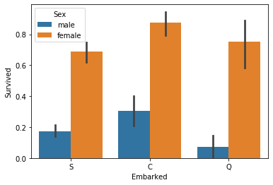
• female的获救率大于 male,(应该是男士都比较绅士吧，即使面对死亡，也希望将最后的机会留给女生，，电影感悟）
• 获救率 C 男性女性都是最高，Q时男性最低，S 时 女性最低
• 男性的获救率低于女性的三分之一

2.2 所做的位置和生存率之间的关系

sns.pointplot(x='Pclass',y='Survived',hue='Sex',data=data_train,palette={'male':'blue','female':'pink'},
             marker=['*',"o"],linestyle=['-','--'])

• 等级越高获救率越高
• 女性大于男性

2.3 生存率与年龄的关系

sns.barplot(x = 'Age',y = 'Survived',hue='Sex',data = data_train)

• 男性大于女性
• student的生存率最低,bady的生存率最高

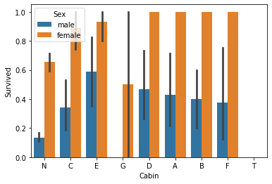
sns.barplot(x = 'Cabin',y = 'Survived',hue='Sex',data = data_train)

sns.barplot(x = 'Fare',y = 'Survived',hue='Sex',data = data_train)

3 建立模型

3.1 随机森林

from sklearn.model_selection import train_test_split
X_all = data_tr.drop(['PassengerId','Survived'],axis=1)#主要是乘客ID也没啥用，删就删了吧
y_all = data_tr['Survived']
p = 0.2 #用 百分之20作为测试集

X_train,X_test, y_train, y_test = train_test_split(X_all,y_all,test_size=p, random_state=23)

from sklearn.ensemble import RandomForestClassifier
from sklearn.metrics import make_scorer, accuracy_score
from sklearn.model_selection import GridSearchCV

#选择分类器的类型，我没试过其他的哦，因为在这个案例中，有人做过试验发现随机森林模型是最好的，所以选了它。呜呜，我下次试试其他的
clf = RandomForestClassifier()

#可以通过定义树的各种参数，限制树的大小，防止出现过拟合现象哦，也可以通过剪枝来限制，但sklearn中的决策树分类器目前不支持剪枝
parameters = {'n_estimators': [4, 6, 9], 
              'max_features': ['log2', 'sqrt','auto'], 
              'criterion': ['entropy', 'gini'],        #分类标准用熵，基尼系数
              'max_depth': [2, 3, 5, 10], 
              'min_samples_split': [2, 3, 5],
              'min_samples_leaf': [1,5,8]
             }

#以下是用于比较参数好坏的评分，使用'make_scorer'将'accuracy_score'转换为评分函数
acc_scorer = make_scorer(accuracy_score)

#自动调参，GridSearchCV，它存在的意义就是自动调参，只要把参数输进去，就能给出最优化的结果和参数
#GridSearchCV用于系统地遍历多种参数组合，通过交叉验证确定最佳效果参数。
grid_obj = GridSearchCV(clf,parameters,scoring=acc_scorer)
grid_obj = grid_obj.fit(X_train,y_train)

#将clf设置为参数的最佳组合
clf = grid_obj.best_estimator_

#将最佳算法运用于数据中
clf.fit(X_train,y_train)

/home/wvdon/anaconda3/envs/weidong/lib/python3.7/site-packages/sklearn/model_selection/_split.py:1978: FutureWarning: The default value of cv will change from 3 to 5 in version 0.22. Specify it explicitly to silence this warning.
  warnings.warn(CV_WARNING, FutureWarning)
/home/wvdon/anaconda3/envs/weidong/lib/python3.7/site-packages/sklearn/model_selection/_search.py:814: DeprecationWarning: The default of the `iid` parameter will change from True to False in version 0.22 and will be removed in 0.24. This will change numeric results when test-set sizes are unequal.
  DeprecationWarning)





RandomForestClassifier(bootstrap=True, class_weight=None, criterion='entropy',
                       max_depth=5, max_features='sqrt', max_leaf_nodes=None,
                       min_impurity_decrease=0.0, min_impurity_split=None,
                       min_samples_leaf=1, min_samples_split=3,
                       min_weight_fraction_leaf=0.0, n_estimators=4,
                       n_jobs=None, oob_score=False, random_state=None,
                       verbose=0, warm_start=False)

3.2 预测

predictions = clf.predict(X_test)
print(accuracy_score(y_test,predictions))
data_tr

0.8268156424581006

	PassengerId	Survived	Pclass	Sex	Age	SibSp	Parch	Fare	Embarked
0	1	0	3	1	22.000000	1	0	7.2500	0
1	2	1	1	0	38.000000	1	0	71.2833	1
2	3	1	3	0	26.000000	0	0	7.9250	0
3	4	1	1	0	35.000000	1	0	53.1000	0
4	5	0	3	1	35.000000	0	0	8.0500	0
...	...	...	...	...	...	...	...	...	...
886	887	0	2	1	27.000000	0	0	13.0000	0
887	888	1	1	0	19.000000	0	0	30.0000	0
888	889	0	3	0	29.699118	1	2	23.4500	0
889	890	1	1	1	26.000000	0	0	30.0000	1
890	891	0	3	1	32.000000	0	0	7.7500	2

891 rows × 9 columns

3.3 预测test文件

predictions = clf.predict(data_te.drop('PassengerId',axis=1))
output = pd.DataFrame({'Passengers':data_te['PassengerId'],'Survived':predictions})
output.to_csv(r'test1.csv')
output.head()

	Passengers	Survived
0	892	0
1	893	0
2	894	0
3	895	0
4	896	0

3.4 提交到kaggle官网

结果是 0.77990
hhhhhhhh还是比较满意的
下次用深度学习试试