TensorFlow应用之进阶版卷积神经网络CNN在CIFAR-10数据集上分类

一、概述

1. 数据集简介

本文使用的数据集是CIFAR-10，这是一个经典的数据集，包含了60000张32*32的彩色图像，其中训练集50000张，测试集10000张，如同其名字，CIFAR-10数据集一共标注为10类，每一类6000张图片，这10类分别是airplane、automobile、bird、cat、deer、dog、frog、horse、ship和truck。类别之间没有重叠，也不会一张图片中出现两类物体，其另一个数据集CIFAR-100则标注了100类。

更多CIFAR相关的信息请参见：http://www.cs.toronto.edu/~kriz/cifar.html

2. 模型简介

在本节的神经网络中，我们采用卷积神经网络CNN，还是用了一些新的技巧：（1）对权重weights进行L2正则化；（2）对图片数据进行数据增强，即对图片进行翻转、随机剪切等操作，制造了更多的样本；（3）在每个卷积-池化层后使用了LRN层（局部相应归一化层），增强了模型的泛化能力。

3. 数据增强DataAugmentation

数据增强在我们的训练中作用很大，包括了随机的水平翻转、随机剪切图片、设置随机的亮度和对比度以及对数据进行标准化等操作。它可以给单幅图增加多个副本，提高图片的利用率，防止对某一个图片结构的学习过拟合。如果神经网络能够克服这些噪声并准确识别，那么其泛化性能必然会很好。

二、程序解读

载入常用库部分首先要添加CIFAR-10相关的cifar10和cifar10_input模块，定义最大迭代轮数max_steps等宏观参数。

定义初始化权重weight的函数，使用截断的正态分布来初始化权重。这里通过一个参数wl来控制对weight的正则化处理。在机器学习中，无论是分类还是回归任务，都可能会因特征过多而导致过拟合问题，一般通过特征选取或惩罚不重要的特征的权重来解决这个问题。但是对于哪些特征是不重要的，我们并不能直观得出，而正则化就是帮助我们惩罚特征权重的，即特征的权重也是损失函数的一部分。可以理解为为了使用某个特征需要付出代价，如果不是这个特征对于减少损失函数非常有效其权重就会被惩罚减小。这样就可以有效的筛选出有效的特征，通过减少特征权重防止过拟合，即奥卡姆剃刀原则（越简单越有效）。L1正则化会制造稀疏的特征，大部分无用的特征直接置为0，而L2正则化会让特征的权重不会过大，使特征的权重比较平均。对于实现L2正则化，有两种方法，tf.multiply(tf.nn.l2_loss(var), wl)其中wl是正则化系数；tf.contrib.layers.l2_regularizer(lambda)(var)其中lambda是正则化系数。

随后使用cifar10模块来下载数据集并解压、展开到默认位置。再用cifar10_input模块来产生数据。其中cifar10_input.distorted_inputs()和cifar10_input.inputs()函数都是TensorFlow的操作operation，操作返回封装好的Tensor，这就需要在会话中run来实际运行。cifar10_input.distorted_inputs()对数据进行了DataAugmentation（数据增强），包括了随机的水平翻转、随机剪切一块24*24的图片、设置随机的亮度和对比度以及对数据进行标准化。通过这些操作，我们可以获得更多的带噪声的样本，扩大了样本容量，对提高准确率有所帮助。需要注意的是，对图像数据进行增强操作会耗费大量的CPU计算时间，因此函数内部使用了16个独立的线程来加速任务，函数内部会产生线程池，在需要时会通过TensorFlow queue进行调度，通过tf.train.start_queue_runners()来启动线程队列。产生测试数据集时则不需要太多操作，仅需要裁剪图片正中间的24*24大小的区块并进行数据标准化操作。

创建第一个卷积层，首先通过variable_with_weight_loss函数创建卷积核的参数并进行初始化，卷积核尺寸为5*5，3个颜色通道，64个卷积核（卷积核深度为64），设置weight初始化标准差为0.05（5e-2），不对第一层卷积层的weight进行L2正则化处理，即wl设为0。在ReLU激活函数之后，我们采用一个3*3的步长为2*2的池化核进行最大池化处理，注意这里最大池化的尺寸和步长不一致，这样可以增加数据的丰富性。随后我们使用tf.nn.lrn()函数，即对结果进行LRN处理。LRN层（局部响应归一化层）模仿了生物神经系统的“侧抑制”机制，对局部神经元的活动创建竞争机制，使得其中响应比较大的值变得相对更大，并抑制其他反馈较小的神经元，增强了模型的泛化能力。LRN对ReLU这种没有上限边界的激活函数比较试用，不适合于Sigmoid这种有固定边界并且能抑制过大值的激活函数。

相似的步骤创建卷积层2，注意权重weight的shape中，通道数为64，bias初始化为0.1，最后的最大池化层和LRN层调换了顺序，先进行LRN层处理后进行最大池化处理。

两个卷积层后使用一个全连接层3，首先将卷积层的输出的样本都reshape为一维向量，获取每个样本的长度后作为全连接层的输入单元数，输出单元数设为384。权重weight初始化并设置L2正则化系数为0.004，我们希望这一层全连接层不要过拟合。

接下来的全连接层4和前一层很像，隐含节点减少一半到192。全连接层5也类似，隐含单元变为最终的分类总数10。

至此，整个网络的inference部分已经完成，网络结构如下表：

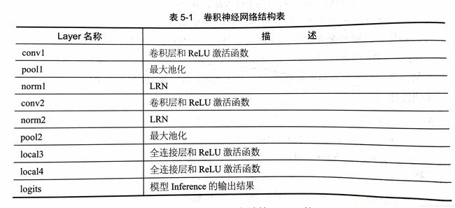
接下来构建CNN'的损失函数loss，定义一个loss函数，tf.add_n()可以将名为losses的collection中的全部loss求和，得到最终包括了cross_entropy的总loss，也包括了后两个全连接层的权重weight的L2 loss。然后定义优化器，定义计算Top K准确率的操作。

下面就是定义会话并进行迭代训练。首先通过session的run方法执行images_train,labels_train来获取每批的训练数据，再将这个batch的训练数据传入train_op和loss的计算，记录每一个step花费的时间。

最后就是在测试集上测评模型的准确率，这里是top1准确率，最得迭代训练3000次后的测评到结果为70.2%。持续增加max_step可以得到更高的准确率。

三、函数使用

1. tf.nn.local_response_normalization / tf.nn.lrn(input,depth_radius=None, bias=None, alpha=None, beta=None, name=None)

input为4-D的Tensor，输出与input相同的Tensor。

sqr_sum[a, b, c,d] = sum(input[a, b, c, d - depth_radius : d + depth_radius + 1] ** 2)

output = input /(bias + alpha * sqr_sum) ** beta

2. tf.nn.in_top_k(predictions, targets, k, name=None)

该函数可以求输出结果中top K的准确率，默认使用top1，即输出分数最高的那一类的准确率。

四、完整代码

import cifar10, cifar10_input
import tensorflow as tf
import numpy as np
import time

max_steps = 3000 # 最大迭代轮数
batch_size = 128 # 批大小
data_dir = 'cifar10_data/cifar-10-batches-bin' # 数据所在路径

# 初始化weight函数，通过wl参数控制L2正则化大小
def variable_with_weight_loss(shape, stddev, wl):
    var = tf.Variable(tf.truncated_normal(shape, stddev=stddev))
    if wl is not None:
        # L2正则化可用tf.contrib.layers.l2_regularizer(lambda)(w)实现，自带正则化参数
        weight_loss = tf.multiply(tf.nn.l2_loss(var), wl, name='weight_loss')
        tf.add_to_collection('losses', weight_loss)
    return var

cifar10.maybe_download_and_extract()
# 此处的cifar10_input.distorted_inputs()和cifar10_input.inputs()函数
# 都是TensorFlow的操作operation，需要在会话中run来实际运行
# distorted_inputs()函数对数据进行了数据增强
images_train, labels_train = cifar10_input.distorted_inputs(data_dir=data_dir,
                                                            batch_size=batch_size)
# 裁剪图片正中间的24*24大小的区块并进行数据标准化操作
images_test, labels_test = cifar10_input.inputs(eval_data=True,
                                                data_dir=data_dir,
                                                batch_size=batch_size)

# 定义placeholder
# 注意此处输入尺寸的第一个值应该是batch_size而不是None
image_holder = tf.placeholder(tf.float32, [batch_size, 24, 24, 3])
label_holder = tf.placeholder(tf.int32, [batch_size])

# 卷积层1，不对权重进行正则化
weight1 = variable_with_weight_loss([5, 5, 3, 64], stddev=5e-2, wl=0.0) # 0.05
kernel1 = tf.nn.conv2d(image_holder, weight1,
                       strides=[1, 1, 1, 1], padding='SAME')
bias1 = tf.Variable(tf.constant(0.0, shape=[64]))
conv1 = tf.nn.relu(tf.nn.bias_add(kernel1, bias1))
pool1 = tf.nn.max_pool(conv1, ksize=[1, 3, 3, 1],
                       strides=[1, 2, 2, 1], padding='SAME')
norm1 = tf.nn.lrn(pool1, 4, bias=1.0, alpha=0.001 / 9.0, beta=0.75)

# 卷积层2
weight2 = variable_with_weight_loss([5, 5, 64, 64], stddev=5e-2, wl=0.0)
kernel2 = tf.nn.conv2d(norm1, weight2, strides=[1, 1, 1, 1], padding='SAME')
bias2 = tf.Variable(tf.constant(0.1, shape=[64]))
conv2 = tf.nn.relu(tf.nn.bias_add(kernel2, bias2))
norm2 = tf.nn.lrn(conv2, 4, bias=1.0, alpha=0.001 / 9.0, beta=0.75)
pool2 = tf.nn.max_pool(norm2, ksize=[1, 3, 3, 1],
                       strides=[1, 2, 2, 1], padding='SAME')

# 全连接层3
reshape = tf.reshape(pool2, [batch_size, -1]) # 将每个样本reshape为一维向量
dim = reshape.get_shape()[1].value # 取每个样本的长度
weight3 = variable_with_weight_loss([dim, 384], stddev=0.04, wl=0.004)
bias3 = tf.Variable(tf.constant(0.1, shape=[384]))
local3 = tf.nn.relu(tf.matmul(reshape, weight3) + bias3)

# 全连接层4
weight4 = variable_with_weight_loss([384, 192], stddev=0.04, wl=0.004)
bias4 = tf.Variable(tf.constant(0.1, shape=[192]))
local4 = tf.nn.relu(tf.matmul(local3, weight4) + bias4)

# 全连接层5
weight5 = variable_with_weight_loss([192, 10], stddev=1 / 192.0, wl=0.0)
bias5 = tf.Variable(tf.constant(0.0, shape=[10]))
logits = tf.matmul(local4, weight5) + bias5

# 定义损失函数loss
def loss(logits, labels):
    labels = tf.cast(labels, tf.int64)
    cross_entropy = tf.nn.sparse_softmax_cross_entropy_with_logits(
            logits=logits, labels=labels, name='cross_entropy_per_example')
    cross_entropy_mean = tf.reduce_mean(cross_entropy, name='cross_entropy')
    tf.add_to_collection('losses', cross_entropy_mean)
    return tf.add_n(tf.get_collection('losses'), name='total_loss')

loss = loss(logits, label_holder) # 定义loss
train_op = tf.train.AdamOptimizer(1e-3).minimize(loss) # 定义优化器
top_k_op = tf.nn.in_top_k(logits, label_holder, 1)

# 定义会话并开始迭代训练
sess = tf.InteractiveSession()
tf.global_variables_initializer().run()
# 启动图片数据增强的线程队列
tf.train.start_queue_runners()

# 迭代训练
for step in range(max_steps):
    start_time = time.time()
    image_batch, label_batch = sess.run([images_train, labels_train]) # 获取训练数据
    _, loss_value = sess.run([train_op, loss],
                             feed_dict={image_holder: image_batch,
                                        label_holder: label_batch})
    duration = time.time() - start_time # 计算每次迭代需要的时间
    if step % 10 == 0:
        examples_per_sec = batch_size / duration # 每秒处理的样本数
        sec_per_batch = float(duration) # 每批需要的时间
        format_str = ('step %d, loss=%.2f (%.1f examples/sec; %.3f sec/batch)')
        print(format_str % (step, loss_value, examples_per_sec, sec_per_batch))

# 在测试集上测评准确率
num_examples = 10000
import math
num_iter = int(math.ceil(num_examples / batch_size))
true_count = 0
total_sample_count = num_iter * batch_size
step = 0
while step < num_iter:
    image_batch, label_batch = sess.run([images_test, labels_test])
    predictions = sess.run([top_k_op],
                           feed_dict={image_holder: image_batch,
                                      label_holder: label_batch})
    true_count += np.sum(predictions)
    step += 1

precision = true_count / total_sample_count
print('precision @ 1 =%.3f' % precision)

'''
step 2900, loss=1.14 (363.7 examples/sec; 0.352 sec/batch)
step 2910, loss=1.05 (372.0 examples/sec; 0.344 sec/batch)
step 2920, loss=1.26 (368.7 examples/sec; 0.347 sec/batch)
step 2930, loss=1.09 (366.4 examples/sec; 0.349 sec/batch)
step 2940, loss=1.02 (366.6 examples/sec; 0.349 sec/batch)
step 2950, loss=1.30 (365.9 examples/sec; 0.350 sec/batch)
step 2960, loss=0.91 (367.1 examples/sec; 0.349 sec/batch)
step 2970, loss=0.96 (364.2 examples/sec; 0.351 sec/batch)
step 2980, loss=1.13 (361.8 examples/sec; 0.354 sec/batch)
step 2990, loss=0.97 (356.0 examples/sec; 0.360 sec/batch)
precision @ 1 =0.702
'''