Machine Learning with Scikit-Learn and Tensorflow 6.8 决策树回归

书籍信息
Hands-On Machine Learning with Scikit-Learn and Tensorflow
出版社: O’Reilly Media, Inc, USA
平装: 566页
语种: 英语
ISBN: 1491962291
条形码: 9781491962299
商品尺寸: 18 x 2.9 x 23.3 cm
ASIN: 1491962291

系列博文为书籍中文翻译
代码以及数据下载：https://github.com/ageron/handson-ml

决策树同样可以实现回归，scikit-learn提供DecisionTreeRegressor利用决策树实现回归，实例如下：

import numpy.random as rnd
from sklearn.tree import DecisionTreeRegressor

# Quadratic training set + noise
rnd.seed(42)
m = 200
X = rnd.rand(m, 1)
y = 4 * (X - 0.5) ** 2
y = y + rnd.randn(m, 1) / 10

# train the decesion tree
tree_reg = DecisionTreeRegressor(random_state=42, max_depth=2)
tree_reg.fit(X, y)

# export the decision tree
export_graphviz(
        tree_reg,
        out_file="regression_tree.dot",
        feature_names=["x1"],
        rounded=True,
        filled=True
    )

译者注：
决策树的可视化参见http://blog.csdn.net/qinhanmin2010/article/details/68499196

实现回归的决策树和实现分类的决策树类似。主要区别是实现分类的决策树预测值是类别，实现回归决策树预测值是数值。例如，根据决策树的可视化结果，如果x1=0.6，那么预测值是0.1106（底部白色结点）。预测值根据110个训练数据的平均值得到，这些数据的mean squared error（MSE）是0.0151。

左图是以上训练的决策树（max_depth=2），右图是max_depth=3的决策树。注意到决策树通过区域内训练数据的平均值得到区域内的预测值，决策树划分区域的依据是使得区域内训练数据的值尽量接近区域内训练数据的平均值。

tree_reg1 = DecisionTreeRegressor(random_state=42, max_depth=2)
tree_reg2 = DecisionTreeRegressor(random_state=42, max_depth=3)
tree_reg1.fit(X, y)
tree_reg2.fit(X, y)

def plot_regression_predictions(tree_reg, X, y, axes=[0, 1, -0.2, 1], ylabel="$y$"):
    x1 = np.linspace(axes[0], axes[1], 500).reshape(-1, 1)
    y_pred = tree_reg.predict(x1)
    plt.axis(axes)
    plt.xlabel("$x_1$", fontsize=18)
    if ylabel:
        plt.ylabel(ylabel, fontsize=18, rotation=0)
    plt.plot(X, y, "b.")
    plt.plot(x1, y_pred, "r.-", linewidth=2, label=r"$\hat{y}$")

plt.figure(figsize=(11, 4))
plt.subplot(121)
plot_regression_predictions(tree_reg1, X, y)
for split, style in ((0.1973, "k-"), (0.0917, "k--"), (0.7718, "k--")):
    plt.plot([split, split], [-0.2, 1], style, linewidth=2)
plt.text(0.21, 0.65, "Depth=0", fontsize=15)
plt.text(0.01, 0.2, "Depth=1", fontsize=13)
plt.text(0.65, 0.8, "Depth=1", fontsize=13)
plt.legend(loc="upper center", fontsize=18)
plt.title("max_depth=2", fontsize=14)

plt.subplot(122)
plot_regression_predictions(tree_reg2, X, y, ylabel=None)
for split, style in ((0.1973, "k-"), (0.0917, "k--"), (0.7718, "k--")):
    plt.plot([split, split], [-0.2, 1], style, linewidth=2)
for split in (0.0458, 0.1298, 0.2873, 0.9040):
    plt.plot([split, split], [-0.2, 1], "k:", linewidth=1)
plt.text(0.3, 0.5, "Depth=2", fontsize=13)
plt.title("max_depth=3", fontsize=14)
plt.show()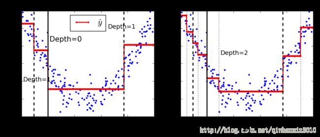

CART算法解决回归问题的思路和解决分类问题类似，不同之处是特征 k 和阈值 tk 的选择依据是最小化以下函数：
J(k,tk)=mleftmMSEleft+mrightmMSEright
其中 MSEleft / MSEright 是子集的mean squared error（参见https://en.wikipedia.org/wiki/Mean_squared_error）， mleft / mright 是子集的训练数据数量。

和分类问题类似，如果不加以限制，那么决策树会尝试精确拟合训练数据，导致过拟合。下面的实例通过构造的数据集说明决策树超参数避免过拟合的作用。左边的决策树没有加以限制，右边的决策树通过min_samples_leaf=10加以限制。可以发现，左边的决策树存在过拟合的问题，右边的决策树效果比较理想。

tree_reg1 = DecisionTreeRegressor(random_state=42)
tree_reg2 = DecisionTreeRegressor(random_state=42, min_samples_leaf=10)
tree_reg1.fit(X, y)
tree_reg2.fit(X, y)

x1 = np.linspace(0, 1, 500).reshape(-1, 1)
y_pred1 = tree_reg1.predict(x1)
y_pred2 = tree_reg2.predict(x1)

plt.figure(figsize=(11, 4))

plt.subplot(121)
plt.plot(X, y, "b.")
plt.plot(x1, y_pred1, "r.-", linewidth=2, label=r"$\hat{y}$")
plt.axis([0, 1, -0.2, 1.1])
plt.xlabel("$x_1$", fontsize=18)
plt.ylabel("$y$", fontsize=18, rotation=0)
plt.legend(loc="upper center", fontsize=18)
plt.title("No restrictions", fontsize=14)

plt.subplot(122)
plt.plot(X, y, "b.")
plt.plot(x1, y_pred2, "r.-", linewidth=2, label=r"$\hat{y}$")
plt.axis([0, 1, -0.2, 1.1])
plt.xlabel("$x_1$", fontsize=18)
plt.title("min_samples_leaf={}".format(tree_reg2.min_samples_leaf), fontsize=14)

plt.show()