【TensorFlow实战笔记】卷积神经网络CNN实战-cifar10数据集(tensorboard可视化)
IDE:pycharm
Python: Python3.6
OS: win10
tf : CPU版本
代码可在github中下载,欢迎star,谢谢 CNN-CIFAR-10
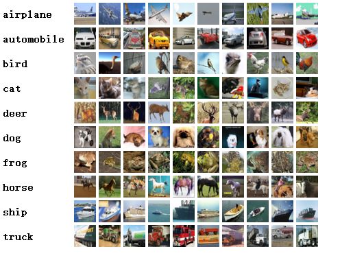
一、CIFAR10数据集
数据集代码下载
from tensorflow.models.tutorials.image.cifar10 import cifar10

cifar10.maybe_download_and_extract()
直接下载数据集的路径为
./tmp/cifar10_data
如果下载不了就直接 官网下载CIFAR-10数据集
下载 CIFAR-10 binary version
放到相应的path,到时候对应即可
官网和网上都有很详细的这个数据集的讲解,基本就是因为是-10所以最后的分类有10类,一种有60000 张32x32三色图片,每种6000张, 50000张train set,10000张test set,还有另外一个孪生数据集CIFAR-100
二、卷积神经网络
卷积神经一般结构:
卷积层+池化层(最大)+全连接层
卷积层和池化层就是最神奇的地方,相当于自动选取特征的过程,也就是提取特征的过程, 全连接层就是输出相应的label,也就是分类的过程。
全连接层又称为多层感知机
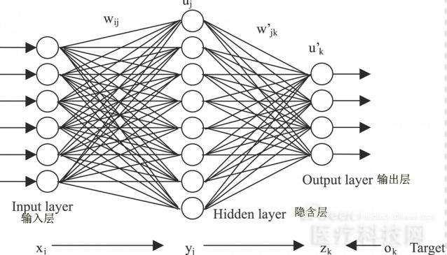
顾名思义就是全连接层的节点与前后层的节点全都有连接。
卷积层和池化层
这里面有一个概念需要知道那就是kernel,有的书里叫做filter
个人觉得filter的概念更容易understand一些

如图所示
- 经过卷积层之后整块矩阵节点会变得
更深,也就是更加深入的分析,从而得到抽象程度更高的特征 - 经过池化层之后矩阵节点的深度没有发生改变,而大小发生改变,可以看成将图片的分辨率变低,主要目的也是让最后与全连接层连接的节点数目变少,从而weights和bias大大减小,加快训练速度
filter过滤器(kernel内核)
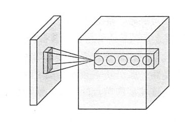
这里假设 矩阵大小是 1281283
现在的fliter的大小 为55(or 33)
- filter中的参数是共享的,这也是使整理的参数减少的策略之一
- 人工除了指定filter的尺寸之外还有就是想得到的新的矩阵的深度
#  5*5大小的fliter 3为前一个矩阵的深度, 16是后一个矩阵的深度
weight = tf.get_variable('weight', shape=[5, 5, 3, 16], initializer=tf.truncated_normal_initializer(stddev=0.1))
#biases的shape就是后一个矩阵的深度
biases = tf.get_variable('biases', [16], initializer=tf.constant_initializer(0.1))
如果是kernel的话就是5*5为kernel的大小, 3为input的深度, 16为kernel的个数
大概的写代码的规律就是这样,还有一个知识点就是stride步长和padding是否补全,这些都是基础,详情参照《Tensorflow实战Google深度学习框架》写的很详细
三、可视化工具 tensorboard
安装tensorflow的时候自动就安装了tensorboard
可视化工具
- Image: 图像
- Audio: 音频
- Histogram: 直方图
- Scalar: 标量
- Graph:计算图
这里面主要使用 后三个
基本使用方法见代码:
 tf.summary.scalar(name, var) #添加scalar量来绘制var
 tf.summary.histogram(name, var)# 添加histogram来绘制var
 #合并全部的summary
 merged = tf.summary.merge_all()
 #写入日志文件和计算图(如果看总体的计算图的话推荐多使用tf.name_scope()划分结构)
 train_writer = tf.summary.FileWriter(LOG_DIR, sess.graph)
 summary, _, loss_value = sess.run([merged, train_op, loss], feed_dict={image_holder: image_batch, label_holder: label_batch})
  #每步进行记录
 train_writer.add_summary(summary, step)
之后再命令台,cd到本项目文件夹
执行
tensorboard --logdir=./LOG
默认 6006 port

记住这里一定要用Chrome浏览器进行浏览就是图中生成的https网站,其他浏览器可能会不好用。
四、总体代码
- 使用cifar10数据集
- 使用cnn网络
- tensorboard可视化
tool.py
"""
@Author:Che_Hongshu
@Function: tools for CNN-CIFAR-10 dataset
@Modify:2018.3.5
@IDE: pycharm
@python :3.6
@os : win10
"""

import tensorflow as tf
"""
函数说明: 得到weights变量和weights的loss
Parameters:
   shape-维度
   stddev-方差
   w1-
Returns:
    var-维度为shape,方差为stddev变量
CSDN:
    http://blog.csdn.net/qq_33431368
Modify:
    2018-3-5
"""
def variable_with_weight_loss(shape, stddev, w1):
    var = tf.Variable(tf.truncated_normal(shape, stddev=stddev))
    if w1 is not None:
        weight_loss = tf.multiply(tf.nn.l2_loss(var), w1, name='weight_loss')
        tf.add_to_collection('losses', weight_loss)
    return var
"""
函数说明: 得到总体的losses
Parameters:
   logits-通过神经网络之后的前向传播的结果
   labels-图片的标签
Returns:
   losses
CSDN:
    http://blog.csdn.net/qq_33431368
Modify:
    2018-3-5
"""
def loss(logits, labels):
    labels = tf.cast(labels, tf.int64)
    cross_entropy = tf.nn.sparse_softmax_cross_entropy_with_logits\
        (logits=logits, labels=labels, name='total_loss')
    cross_entropy_mean = tf.reduce_mean(cross_entropy, name='cross_entorpy')
    tf.add_to_collection('losses', cross_entropy_mean)
    return tf.add_n(tf.get_collection('losses'), name='total_loss')

"""
函数说明: 对变量进行min max 和 stddev的tensorboard显示
Parameters:
    var-变量
    name-名字
Returns:
    None
CSDN:
    http://blog.csdn.net/qq_33431368
Modify:
    2018-3-5
"""
def variables_summaries(var, name):
    with tf.name_scope('summaries'):
        mean = tf.reduce_mean(var)
        tf.summary.scalar('mean/'+name, mean)
        with tf.name_scope('stddev'):
            stddev = tf.sqrt(tf.reduce_sum(tf.square(var-mean)))
        tf.summary.scalar('stddev/' + name, stddev)
        tf.summary.scalar('max/' + name, tf.reduce_max(var))
        tf.summary.scalar('min/' + name, tf.reduce_min(var))
        tf.summary.histogram(name, var)
        tf.summary.histogram()
CNN:
"""
@Author:Che_Hongshu
@Function: CNN-CIFAR-10 dataset
@Modify:2018.3.5
@IDE: pycharm
@python :3.6
@os : win10
"""
from tensorflow.models.tutorials.image.cifar10 import cifar10
from tensorflow.models.tutorials.image.cifar10 import cifar10_input

import tensorflow as tf
import numpy as np
import time
import tools
max_steps = 3000 # 训练轮数
batch_size = 128  #一个bacth的大小
data_dir = './cifar-10-batches-bin' #读取数据文件夹
LOG_DIR = './LOG'

#下载CIFAR数据集 如果不好用直接
# http://www.cs.toronto.edu/~kriz/cifar.html 下载CIFAR-10 binary version 文件解压放到相应的文件夹中
#cifar10.maybe_download_and_extract()
#得到训练集的images和labels
#print(images_train) 可知是一个shape= [128, 24, 24, 3]的tensor
images_train, labels_train = cifar10_input.\
    distorted_inputs(data_dir=data_dir, batch_size=batch_size)
#得到测试集的images和labels
images_test, labels_test = cifar10_input.\
    inputs(eval_data=True, data_dir=data_dir, batch_size=batch_size)
#以上两个为什么分别用distorted_inputs and inputs  请go to definition查询
#创建输入数据的placeholder
with tf.name_scope('input_holder'):
    image_holder = tf.placeholder(tf.float32, [batch_size, 24, 24, 3])
    label_holder = tf.placeholder(tf.int32, [batch_size])
#下面的卷积层的 weights的l2正则化不计算, 一般只在全连接层计算正则化loss
#第一个conv层
#5*5的卷积核大小,3个channel ,64个卷积核, weight的标准差为0.05
with tf.name_scope('conv1'):
    #加上更多的name_scope 使graph更加清晰好看,代码也更加清晰
    with tf.name_scope('weight1'): #权重
        weight1 = tools.variable_with_weight_loss(shape=[5, 5, 3, 64], stddev=5e-2, w1=0.0)
        #运用tensorboard进行显示
        tools.variables_summaries(weight1, 'conv1/weight1')
    kernel1 = tf.nn.conv2d(image_holder, weight1, strides=[1, 1, 1, 1], padding='SAME')
    with tf.name_scope('bias1'): #偏置
        bias1 = tf.Variable(tf.constant(0.0, shape=[64]))
        tools.variables_summaries(bias1, 'conv1/bias1')
    with tf.name_scope('forward1'): #经过这个神经网络的前向传播的算法结果
        conv1 = tf.nn.relu(tf.nn.bias_add(kernel1, bias1))#cnn加上bias需要调用bias_add不能直接+
#第一个最大池化层和LRN层
with tf.name_scope('pool_norm1'):
    with tf.name_scope('pool1'):
        # ksize和stride不同 , 多样性
        pool1 = tf.nn.max_pool(conv1, ksize=[1, 2, 2, 1], strides=[1, 3, 3, 1], padding='SAME')
    with tf.name_scope('LRN1'):
        #LRN层可以使模型更加
        norm1 = tf.nn.lrn(pool1, 4, bias=1.0, alpha=0.001/9.0, beta=0.75)

#第二层conv层 input: 64   size = 5*5   64个卷积核
with tf.name_scope('conv2'):
    with tf.name_scope('weight2'):
        weight2 = tools.variable_with_weight_loss(shape=[5, 5, 64, 64], stddev=5e-2, w1=0.0)
        tools.variables_summaries(weight2, 'conv2/weight2')
    kernel2 = tf.nn.conv2d(norm1, weight2, strides=[1, 1, 1, 1], padding='SAME')
    with tf.name_scope('bias2'):
        bias2 = tf.Variable(tf.constant(0.1, shape=[64]))
        tools.variables_summaries(bias2, 'conv2/bias2')
    with tf.name_scope('forward2'):
        conv2 = tf.nn.relu(tf.nn.bias_add(kernel2, bias2))

#第二个LRN层和最大池化层
with tf.name_scope('norm_pool2'):
    with tf.name_scope('LRN2'):
        norm2 = tf.nn.lrn(conv2, 4, bias=1.0, alpha=0.001/9.0, beta=0.75)
    with tf.name_scope('pool2'):
        pool2 = tf.nn.max_pool(norm2, ksize=[1, 3, 3, 1], strides=[1, 2, 2, 1], padding='SAME')
# 全连接网络
with tf.name_scope('fnn1'):
    reshape = tf.reshape(pool2, [batch_size, -1])
    dim = reshape.get_shape()[1].value
    with tf.name_scope('weight3'):
        weight3 = tools.variable_with_weight_loss(shape=[dim, 384], stddev=0.04, w1=0.004)
        tools.variables_summaries(weight3, 'fnn1/weight3')
    with tf.name_scope('bias3'):
        bias3 = tf.Variable(tf.constant(0.1, shape=[384]))
        tools.variables_summaries(bias3, 'fnn1/bias3')
    local3 = tf.nn.relu(tf.matmul(reshape, weight3) + bias3)

with tf.name_scope('fnn2'):
    with tf.name_scope('weight4'):
        weight4 = tools.variable_with_weight_loss(shape=[384, 192], stddev=0.04, w1=0.004)
    with tf.name_scope('bias4'):
        bias4 = tf.Variable(tf.constant(0.1, shape=[192]))
    local4 = tf.nn.relu(tf.matmul(local3, weight4) + bias4)
with tf.name_scope('inference'):
    with tf.name_scope('weight5'):
        weight5 = tools.variable_with_weight_loss(shape=[192, 10], stddev=1/192.0, w1=0.0)
    with tf.name_scope('bias5'):
        bias5 = tf.Variable(tf.constant(0.0, shape=[10]))
    logits = tf.add(tf.matmul(local4, weight5), bias5)


with tf.name_scope('loss_func'):
    #求出全部的loss
    loss = tools.loss(logits, label_holder)
    tf.summary.scalar('loss', loss)

with tf.name_scope('train_step'):
	step = tf.train.get_or_create_global_step()
    #调用优化方法Adam,这里学习率是直接设定的自行可以decay尝试一下
    train_op = tf.train.AdamOptimizer(1e-3).minimize(loss, global_step=step)
    top_k_op = tf.nn.in_top_k(logits, label_holder, 1)

#创建会话
sess = tf.InteractiveSession()
#变量初始化
tf.global_variables_initializer().run()
#合并全部的summary
merged = tf.summary.merge_all()
#将日志文件写入LOG_DIR中
train_writer = tf.summary.FileWriter(LOG_DIR, sess.graph)
#因为数据集读取需要打开线程,这里打开线程
tf.train.start_queue_runners()
#开始迭代训练
for step in range(max_steps):
    start_time = time.time()
    image_batch, label_batch = sess.run([images_train, labels_train])
    summary, _, loss_value = sess.run([merged, train_op, loss], feed_dict={image_holder: image_batch, label_holder: label_batch})
    #每步进行记录
    train_writer.add_summary(summary, step)
    duration = time.time() - start_time
    if step % 10 == 0:
        examples_per_sec = batch_size / duration
        #训练一个batch的time
        sec_per_batch = float(duration)
        format_str = ('step %d, loss=%.2f (%.1f examples/sec; %.3f sec/batch)')
        print(format_str % (step, loss_value, examples_per_sec, sec_per_batch))

num_examples = 10000
import math
num_iter = int(math.ceil(num_examples/batch_size))
true_count = 0
total_sample_count = num_iter * batch_size
step = 0
while step < num_iter:
    image_batch, label_batch = sess.run([images_test, labels_test])
    predictions = sess.run([top_k_op], feed_dict={image_holder: image_batch, label_holder: label_batch})
    true_count += np.sum(predictions)
    step += 1
precision = true_count/total_sample_count

print('precision = %.3f' % precision)
五、结果分析
大概经过20分钟左右吧,关键还得看你的电脑和你的tf的版本我的是CPU版本比较慢,建议用linux的GPU版本。
1.程序结果
[外链图片转存失败,源站可能有防盗链机制,建议将图片保存下来直接上传(img-nQ7S5fcB-1571489621323)(https://img-blog.csdn.net/20180305234129693?watermark/2/text/aHR0cDovL2Jsb2cuY3Nkbi5uZXQvcXFfMzM0MzEzNjg=/font/5a6L5L2T/fontsize/400/fill/I0JBQkFCMA==/dissolve/70)]
测试集之后的acc比较低,因为我们没有其他的trick,比如learning decay之类的。
2. tensorboard的可视化
输入之后打开Chrome浏览器进入tensorboard
上面为各个指标的显示形式的选择,右下方为conv1的参数变化
CONV2:
[外链图片转存失败,源站可能有防盗链机制,建议将图片保存下来直接上传(img-FYA9oTZR-1571489621324)(https://img-blog.csdn.net/201803052348062?watermark/2/text/aHR0cDovL2Jsb2cuY3Nkbi5uZXQvcXFfMzM0MzEzNjg=/font/5a6L5L2T/fontsize/400/fill/I0JBQkFCMA==/dissolve/70)]
FNN1:
[外链图片转存失败,源站可能有防盗链机制,建议将图片保存下来直接上传(img-TNip5chG-1571489621324)(https://img-blog.csdn.net/20180305235021181?watermark/2/text/aHR0cDovL2Jsb2cuY3Nkbi5uZXQvcXFfMzM0MzEzNjg=/font/5a6L5L2T/fontsize/400/fill/I0JBQkFCMA==/dissolve/70)]
loss:(一般分析主要看loss loss减小的越小越好)
[外链图片转存失败,源站可能有防盗链机制,建议将图片保存下来直接上传(img-gl7r7vax-1571489621325)(https://img-blog.csdn.net/20180305235122324?watermark/2/text/aHR0cDovL2Jsb2cuY3Nkbi5uZXQvcXFfMzM0MzEzNjg=/font/5a6L5L2T/fontsize/400/fill/I0JBQkFCMA==/dissolve/70)]
IMAGES:
HISTOGRAMS
[外链图片转存失败,源站可能有防盗链机制,建议将图片保存下来直接上传(img-xoe1olLL-1571489621325)(https://img-blog.csdn.net/20180305235339122?watermark/2/text/aHR0cDovL2Jsb2cuY3Nkbi5uZXQvcXFfMzM0MzEzNjg=/font/5a6L5L2T/fontsize/400/fill/I0JBQkFCMA==/dissolve/70)]
其他的自行观看即可这里不再过多介绍
计算图的框图:
[外链图片转存失败,源站可能有防盗链机制,建议将图片保存下来直接上传(img-kjvDKY6H-1571489621325)(https://img-blog.csdn.net/20180305235458265?watermark/2/text/aHR0cDovL2Jsb2cuY3Nkbi5uZXQvcXFfMzM0MzEzNjg=/font/5a6L5L2T/fontsize/400/fill/I0JBQkFCMA==/dissolve/70)]
讲道理不知道为啥这么丑。。。
之后每个带+号的都可以展开
比如
conv2:
over。