模型可解释性

模型可解释性：使用机器学习可解释性工具解释心脏病原因

五部分内容：

1. 简介
2. 数据
3. 模型
4. 解释
5. 总结

1. 介绍

纵观机器学习的所有应用，当使用黑盒子模型去进行重要疾病诊断时总是难以让人信服。如果诊断模型的输出是一系列的特殊治疗过程（可能有副作用），比如需要手术，或者不需要治疗，人们总想知道为什么会有这样的结果，想知道模型输出的原因。
这个数据集包含了很多有心脏病和没有心脏病的样本，每个样本包含很多与疾病相关的特征变量。以下采用的是一个简单的随机森林模型，然后用模型可解释性工具和技术深入研究。
具体代码和解释，首先加载相应的库：

import numpy as np
import pandas as pd
import matplotlib.pyplot as plt
import seaborn as sns #for plotting
from sklearn.ensemble import RandomForestClassifier #for the model
from sklearn.tree import DecisionTreeClassifier
from sklearn.tree import export_graphviz #plot tree
from sklearn.metrics import roc_curve, auc #for model evaluation
from sklearn.metrics import classification_report #for model evaluation
from sklearn.metrics import confusion_matrix #for model evaluation
from sklearn.model_selection import train_test_split #for data splitting
import eli5 #for permutation importance
from eli5.sklearn import PermutationImportance
import shap #for SHAP values
from pdpbox import pdp, info_plots #for partial plots
np.random.seed(123) #ensure reproducibility

pd.options.mode.chained_assignment = None  #hide any pandas warnings

2. 数据

加载数据和分析数据

dt = pd.read_csv("../input/heart.csv")

查看数据内容

dt.head(10)

	age	sex	cp	trestbps	chol	fbs	restecg	thalach	exang	oldpeak	slope	ca	thal	target
0	63	1	3	145	233	1	0	150	0	2.3	0	0	1	1
1	37	1	2	130	250	0	1	187	0	3.5	0	0	2	1
2	41	0	1	130	204	0	0	172	0	1.4	2	0	2	1
3	56	1	1	120	236	0	1	178	0	0.8	2	0	2	1
4	57	0	0	120	354	0	1	163	1	0.6	2	0	2	1
5	57	1	0	140	192	0	1	148	0	0.4	1	0	1	1
6	56	0	1	140	294	0	0	153	0	1.3	1	0	2	1
7	44	1	1	120	263	0	1	173	0	0.0	2	0	3	1
8	52	1	2	172	199	1	1	162	0	0.5	2	0	3	1
9	57	1	2	150	168	0	1	174	0	1.6	2	0	2	1

数据内容简单清晰，以下是其中每一列的具体含义：

age：年龄

sex：性别（1=男，0=女）

cp：胸部疼痛经历（1：典型性心绞痛，2：非典型型心绞痛，3：无心绞痛,4:无心绞痛）

trestbps：休息时血压（mm Hg）

chol：胆固醇含量（mg/dl）

fbs：空腹血糖含量（>120mg/dl, 1=true,0=false）

restecg：静息心电图测量（0=正常，1=st-t波异常，2=根据Extes标准，可能左心房肥厚）

thalach：最大心率

exang：运动诱发心绞痛（1=yes,0=no）

oldpeak：由运动引起st段下降（心电图）

slope：峰值ST段的斜率（1：上斜,2:平坦,3:下斜）

ca：大血管数量（0-3）

thal：地中海贫血（3=正常，6=固定缺陷，7=可逆缺陷）

target：是否心脏病（0=no，1=yes）

为了避免事后诸葛亮，我们提前查阅心脏病的诊断指导，并且对比上述特征。

诊断：

心脏病诊断

医学测试

风险存在

预防心脏病

从上述中没有找到对应大血管这一特征，但是心脏病的定义跟大血管有关“…当你的心脏血液供应被冠状动脉中的脂肪物质阻塞或中断时…”，看起来是有关系的。

根据上述查阅，我们可以假设，如果这个模型是由预测能力的，那么这些因素都会有各自的影响因子

将上述特征写成一列，表述更清晰：

dt.columns=['age', 'sex', 'chest_pain_type', 'resting_blood_pressure', 'cholesterol', 'fasting_blood_sugar', 'rest_ecg', 'max_heart_rate_achieved',
       'exercise_induced_angina', 'st_depression', 'st_slope', 'num_major_vessels', 'thalassemia', 'target']

为了后边表述清楚，将数字表达转换为特征名字

# sex
dt['sex'][dt['sex']==0]='female'
dt['sex'][dt['sex']==1]='male'
# cp
dt['chest_pain_type'][dt['chest_pain_type'] == 1] = 'typical angina'
dt['chest_pain_type'][dt['chest_pain_type'] == 2] = 'atypical angina'
dt['chest_pain_type'][dt['chest_pain_type'] == 3] = 'non-anginal pain'
dt['chest_pain_type'][dt['chest_pain_type'] == 4] = 'asymptomatic'
# fbs
dt['fasting_blood_sugar'][dt['fasting_blood_sugar']==0]= 'lower than 120mg/ml'
dt['fasting_blood_sugar'][dt['fasting_blood_sugar'] == 1] = 'greater than 120mg/ml'
#restecg
dt['rest_ecg'][dt['rest_ecg'] == 0] = 'normal'
dt['rest_ecg'][dt['rest_ecg'] == 1] = 'ST-T wave abnormality'
dt['rest_ecg'][dt['rest_ecg'] == 2] = 'left ventricular hypertrophy'
# exang
dt['exercise_induced_angina'][dt['exercise_induced_angina'] == 0] = 'no'
dt['exercise_induced_angina'][dt['exercise_induced_angina'] == 1] = 'yes'
# slope
dt['st_slope'][dt['st_slope'] == 1] = 'upsloping'
dt['st_slope'][dt['st_slope'] == 2] = 'flat'
dt['st_slope'][dt['st_slope'] == 3] = 'downsloping'
# thal
dt['thalassemia'][dt['thalassemia'] == 1] = 'normal'
dt['thalassemia'][dt['thalassemia'] == 2] = 'fixed defect'
dt['thalassemia'][dt['thalassemia'] == 3] = 'reversable defect'

dt.dtypes

age                          int64
sex                         object
chest_pain_type             object
resting_blood_pressure       int64
cholesterol                  int64
fasting_blood_sugar         object
rest_ecg                    object
max_heart_rate_achieved      int64
exercise_induced_angina     object
st_depression              float64
st_slope                    object
num_major_vessels            int64
thalassemia                 object
target                       int64
dtype: object

其中的一些是不对的。以下代码保证变为分类变量

dt['sex'] = dt['sex'].astype('object')
dt['chest_pain_type'] = dt['chest_pain_type'].astype('object')
dt['fasting_blood_sugar'] = dt['fasting_blood_sugar'].astype('object')
dt['rest_ecg'] = dt['rest_ecg'].astype('object')
dt['exercise_induced_angina'] = dt['exercise_induced_angina'].astype('object')
dt['st_slope'] = dt['st_slope'].astype('object')
dt['thalassemia'] = dt['thalassemia'].astype('object')

dt.dtypes

age                          int64
sex                         object
chest_pain_type             object
resting_blood_pressure       int64
cholesterol                  int64
fasting_blood_sugar         object
rest_ecg                    object
max_heart_rate_achieved      int64
exercise_induced_angina     object
st_depression              float64
st_slope                    object
num_major_vessels            int64
thalassemia                 object
target                       int64
dtype: object

dt.head()

	age	sex	chest_pain_type	resting_blood_pressure	cholesterol	fasting_blood_sugar	rest_ecg	max_heart_rate_achieved	exercise_induced_angina	st_depression	st_slope	num_major_vessels	thalassemia	target
0	63	male	non-anginal pain	145	233	greater than 120mg/ml	normal	150	no	2.3	0	0	normal	1
1	37	male	atypical angina	130	250	lower than 120mg/ml	ST-T wave abnormality	187	no	3.5	0	0	fixed defect	1
2	41	female	typical angina	130	204	lower than 120mg/ml	normal	172	no	1.4	flat	0	fixed defect	1
3	56	male	typical angina	120	236	lower than 120mg/ml	ST-T wave abnormality	178	no	0.8	flat	0	fixed defect	1
4	57	female	0	120	354	lower than 120mg/ml	ST-T wave abnormality	163	yes	0.6	flat	0	fixed defect	1

对于分类变量，我们需要创建虚拟变量，并且丢掉每类的描述特征，如用’0’,'1’表示男性和女性

dt=pd.get_dummies(dt,drop_first=True)

dt.head()

	age	resting_blood_pressure	cholesterol	max_heart_rate_achieved	st_depression	num_major_vessels	target	sex_male	chest_pain_type_atypical angina	chest_pain_type_non-anginal pain	chest_pain_type_typical angina	fasting_blood_sugar_lower than 120mg/ml	rest_ecg_left ventricular hypertrophy	rest_ecg_normal	exercise_induced_angina_yes	st_slope_flat	st_slope_upsloping	thalassemia_fixed defect	thalassemia_normal	thalassemia_reversable defect
0	63	145	233	150	2.3	0	1	1	0	1	0	0	0	1	0	0	0	0	1	0
1	37	130	250	187	3.5	0	1	1	1	0	0	1	0	0	0	0	0	1	0	0
2	41	130	204	172	1.4	0	1	0	0	0	1	1	0	1	0	1	0	1	0	0
3	56	120	236	178	0.8	0	1	1	0	0	1	1	0	0	0	1	0	1	0	0
4	57	120	354	163	0.6	0	1	0	0	0	0	1	0	0	1	1	0	1	0	0

这样子看起来好多了，下边介绍模型

3. 模型

采用随机森林对数据建模

X_train, X_test, y_train, y_test = train_test_split(dt.drop('target', 1), dt['target'], test_size = .2, random_state=10) #split the data

model = RandomForestClassifier(max_depth=5)
model.fit(X_train, y_train)

RandomForestClassifier(bootstrap=True, class_weight=None, criterion='gini',
            max_depth=5, max_features='auto', max_leaf_nodes=None,
            min_impurity_decrease=0.0, min_impurity_split=None,
            min_samples_leaf=1, min_samples_split=2,
            min_weight_fraction_leaf=0.0, n_estimators=10, n_jobs=None,
            oob_score=False, random_state=None, verbose=0,
            warm_start=False)

绘制顺向决策树，查看做了什么

estimator = model.estimators_[1]
feature_names = [i for i in X_train.columns]

y_train_str = y_train.astype('str')
y_train_str[y_train_str == '0'] = 'no disease'
y_train_str[y_train_str == '1'] = 'disease'
y_train_str = y_train_str.values

#code from https://towardsdatascience.com/how-to-visualize-a-decision-tree-from-a-random-forest-in-python-using-scikit-learn-38ad2d75f21c
export_graphviz(estimator,out_file='tree.dot',
               feature_names = feature_names,
               class_names = y_train_str,
               rounded = True, proportion = True,
               label='root',
               precision = 2,filled = True)

from subprocess import call
call(['dot', '-Tpng', 'tree.dot', '-o', 'tree.png', '-Gdpi=600'])
from IPython.display import Image
Image(filename='tree.png')

如果上述文件打不开，则需要到指定路径下如，打开cmd，到’E:\work\kaggle\March\aikeke_heart\code’下，输入
dot -Tpng tree.dot -o tree.png，则会生成tree.png
参考dot解决

这提供给我们一个解释性工具，然而，我们不能一眼看出最重要的特征是什么，稍后我们会继续分析。接下来评估这个模型

y_predict = model.predict(X_test)
y_pred_quant = model.predict_proba(X_test)[:, 1]
y_pred_bin = model.predict(X_test)

我们用混淆矩阵来估计这个模型

confusion_matrix = confusion_matrix(y_test, y_pred_bin)
confusion_matrix

array([[28,  7],
       [ 3, 23]], dtype=int64)

疾病诊断的两个常用评估准则是灵敏度和特异性：
灵敏度（sensitivity），又称真阳性率，即实际有病，并且按照该诊断试验的标准被正确地判为有病的百分比。它反映了诊断试验发现病人的能力。

特异性（specificity），又称真阴性率，即实际没病，同时被诊断试验正确地判为无病的百分比。它反映了诊断试验确定非病人的能力。

正确判断病人的率:
$$灵敏度=真阳性人数TP/（真阳性人数TP+假阴性人数FN）\ast 100$$
正确判断非病人的率:
$$特异性=真阴性人数TN/（真阴性人数TN+假阳性人数FP）\ast 100$$

total=sum(sum(confusion_matrix))

sensitivity = confusion_matrix[0,0]/(confusion_matrix[0,0]+confusion_matrix[1,0])
print('Sensitivity : ', sensitivity )

specificity = confusion_matrix[1,1]/(confusion_matrix[1,1]+confusion_matrix[0,1])
print('Specificity : ', specificity)

Sensitivity :  0.9032258064516129
Specificity :  0.7666666666666667

查看ROC曲线

fpr,tpr,thresholds = roc_curve(y_test, y_pred_quant)

fig, ax =plt.subplots()
ax.plot(fpr,tpr)
ax.plot([0, 1], [0, 1], transform=ax.transAxes, ls="--", c=".3")
plt.xlim([0.0, 1.0])
plt.ylim([0.0, 1.0])
plt.rcParams['font.size'] = 12
plt.title('ROC curve for diabetes classifier')
plt.xlabel('False Positive Rate (1 - Specificity)')
plt.ylabel('True Positive Rate (Sensitivity)')
plt.grid(True)

另一个常用的度量是AUC(曲线下的面积)。这是用单个数字捕获模型性能的一种方法。根据经验，AUC可以分类如下

0.90 - 1.00 = excellent

0.80 - 0.90 = good

0.70 - 0.80 = fair

0.60 - 0.70 = poor

0.50 - 0.60 = fail

auc(fpr, tpr)

0.9131868131868132

4. 解释

现在我们看看通过模型解释可以从模型获取那些信息
Permutation importance是我们理解机器学习模型的第一个工具，它涉及到对验证集数据中变量打乱顺序(在拟合模型之后)，并观察其对准确性的影响。

perm = PermutationImportance(model, random_state=1).fit(X_test, y_test)
eli5.show_weights(perm, feature_names = X_test.columns.tolist())

从重要性排列来看，最重要的因素是“可逆转缺陷”导致的thalessemia（地中海贫血），max_heart_rate_achieved（最大心率）的高度重要性也是有理由的，这是患者在检查时最直接的主观状态(而不是年龄，年龄是一个更普遍的因素)。

下边我们使用Partial Dependence Plot查看 num_major_vessels（大血管数量）。这些图来自于改变单一变量在一个值范围内时对输出结果的影响。我们来看看’ num_major_servers '变量带来的影响

base_features = dt.columns.values.tolist()
base_features.remove('target')#delete the target from the list
feat_name = 'num_major_vessels'
pdp_dist = pdp.pdp_isolate(model=model, dataset=X_test, model_features=base_features, feature=feat_name)

pdp.pdp_plot(pdp_dist, feat_name)
plt.show()

可以看到，随着 num_major_vessels（大血管数量）的增加，心脏病率减少，这个在情理之中，因为它意味着更多的血液可以到达心脏而不会堵塞，那么下边查看age（年龄）

feat_name = 'age'
pdp_dist = pdp.pdp_isolate(model=model, dataset=X_test, model_features=base_features, feature=feat_name)

pdp.pdp_plot(pdp_dist, feat_name)
plt.show()

看起来有点奇怪，好像是年纪越大越不容易患心脏病，尽管蓝色区域表明这个可能不准确（红色基准线在蓝色区域内），那么st_depression（运动引起ST段下降）的影响呢？

feat_name = 'st_depression'
pdp_dist = pdp.pdp_isolate(model=model, dataset=X_test, model_features=base_features, feature=feat_name)

pdp.pdp_plot(pdp_dist, feat_name)
plt.show()

有趣的是，这个变量越高，患病概率也越低。这是什么意思呢?通过在谷歌上的搜索，得到了以下描述:Anthony L. Komaroff：医学博士，一位内科专家“心电图(ECG)测量心脏的电活动。出现在上面的波被标记为P、QRS和T，每一个都对应心跳的不同部分,ST段代表右心室和左心室收缩后心脏的电活动，将血液送进肺和身体其他部位。跟随这一巨大的努力，心室肌细胞放松，为下一次收缩做好准备。在此期间，几乎没有电流流动，因此ST段与基线持平，有时略高于基线。心脏跳动得越快，心电图检测时所有的波就变得越短。ST段的形状和方向远比它的长度重要。向上或向下的变化可以表示流向心脏的血液减少有多种原因,包括心脏病、冠状动脉痉挛(Prinzmetal心绞痛)，心脏内壁,感染(心包炎)或心肌本身(心肌炎),血液中有过多的钾,心脏节律的问题,或肺中血凝块(肺栓塞)。

这个变量，被描述为“运动相对于休息引起的ST段下降”，似乎表明这个值越高，患心脏病的概率就越高，但是上面的图表显示的是相反的。也许重要的不只是下降程度，还有与斜率类型的相互作用?让我们用2D PDP检查验证

inter1  =  pdp.pdp_interact(model=model, dataset=X_test, model_features=base_features, features=['st_slope_upsloping', 'st_depression'])

pdp.pdp_interact_plot(pdp_interact_out=inter1, feature_names=['st_slope_upsloping', 'st_depression'], plot_type='contour')
plt.show()

inter1  =  pdp.pdp_interact(model=model, dataset=X_test, model_features=base_features, features=['st_slope_flat', 'st_depression'])

pdp.pdp_interact_plot(pdp_interact_out=inter1, feature_names=['st_slope_flat', 'st_depression'], plot_type='contour')
plt.show()

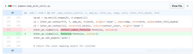
在绘制上图的过程中出现有问题：

TypeError: clabel() got an unexpected keyword argument ‘contour_label_fontsize’

解决方法：

看起来ST段下降在这两种情况下都是不好的。让我们看看SHAP值告诉我们什么。这些工作通过对比单个变量与它们的基准值来观察对结果的影响。

explainer = shap.TreeExplainer(model)
shap_values = explainer.shap_values(X_test)

shap.summary_plot(shap_values[1], X_test, plot_type="bar")

shap.summary_plot(shap_values[1], X_test)

大血管数量的划分是很清楚的，数量越少越不好(右边的蓝色)。地中海贫血“可逆转缺陷”的划分非常清晰(yes =红色=好，no =蓝色=坏)。

你可以在许多其他变量中看到一些明显的分离。运动诱发的心绞痛有明显的分离，虽然不像预期的那样，因为“no”(蓝色)增加了概率。
另一个明显的是st_slope。当它看起来是平坦时是个不好的信号(右边的红色)。

同样奇怪的是，在这个模型中，男性(红色)患心脏病的几率较低。这是为什么呢?专业知识告诉我们的时男人有更大的概率患病。
接下来，让我们挑出个别的病人看看不同的变量是如何影响他们的结果。

def heart_disease_risk_factors(model,patient):
    explainer = shap.TreeExplainer(model)
    shap_values = explainer.shap_values(patient)
    shap.initjs()
    return shap.force_plot(explainer.expected_value[1], shap_values[1], patient)
    

对于这个人来说，他的预测是36%(相比之下基线是58.4%)。许多事情都对他们有利，包括有一个大的血管，一个可逆的地中海贫血缺陷，没有一个平坦的st_slope。让我们查看另一个。

data_for_prediction = X_test.iloc[1,:].astype(float)
heart_disease_risk_factors(model, data_for_prediction)

data_for_prediction = X_test.iloc[3,:].astype(float)
heart_disease_risk_factors(model, data_for_prediction)

对于这个人来说，他的预测是70%(相比之下基线是58.4%)。对他不利的因素包括没有大血管，st_slope平坦，以及不可逆的地中海贫血。
我们还可以绘制所谓的“SHAP依赖贡献图”，在SHAP值shap的描述中，这是不言自明的。

ax2 = fig.add_subplot(224)
shap.dependence_plot('num_major_vessels', shap_values[1], X_test, interaction_index="st_depression")

可以看到血管数量具有明显的影响，但是st_depression（不同颜色表示值）似乎并没有太大的影响。

最后一个图对于我来说，是最有效的一个。它显示了对许多(在本例中是50名)患者预测结果的影响因素。这个图是很好的互动图。可以将鼠标悬停在屏幕上，看看为什么每个人最后要么是红色(疾病预测)，要么是蓝色(没有疾病预测)。

shap_values = explainer.shap_values(X_train.iloc[:50])
shap.force_plot(explainer.expected_value[1], shap_values[1], X_test.iloc[:50])

5. 总结

以今天的标准来看，这个数据集又旧又小。然而，它允许我们创建一个简单的模型，然后使用各种机器学习解释工具和技术来深入研究。一开始，我使用谷歌搜索领域知识进行假设，认为胆固醇和年龄等因素将是模型中的主要因素。然而数据集并没有显示这一点，相反，心电图的结果时主要因素和大血管的数量占主导地位。我认为，随着机器学习在健康医疗和金融预测中发挥越来越大的作用，这种方法将变得越来越重要。

参考文件：
what causes heart disease
https://arxiv.org/pdf/1706.06060.pdf