分类问题(Classification)
在分类问题中,我们尝试预测离散值输出,例如:判断一封电子邮件是否为垃圾邮件、判断一次在线交易是否为诈骗和判断肿瘤是否为恶性肿瘤等。
我们先从二元分类问题(即预测结果为0和1)开始讨论。我们将要预测的因变量y的取值分为两类:当y=1时,我们将其标记为正向类(Positive Class);当y=0时,我们将其标记为负向类(Negative Class)。
因此,因变量y可用数学符号记为:y∈{0, 1},其中0表示负向类,1表示正向类。
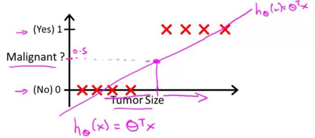
现在,我们再来回顾一下之前的肿瘤预测这个例子。假设我们有如下数据集,我们根据之前学习的线性回归的知识,可以用一条直线来帮助我们预测肿瘤是否为恶性肿瘤。
根据这条直线,我们可以将分类器的输出阀值设置为0.5,即:
按照上述操作,数据集右侧的数据都为正向类,左侧的数据都为负向类。
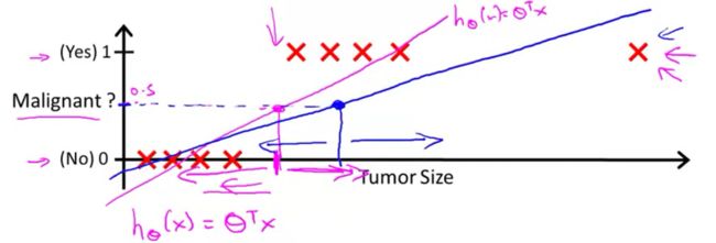
这时,我们延长数据集的横轴并添加一个训练数据。
根据之前的判断,数据集中存在某一个值(肿瘤大小)使得假设函数h的值恰好为阀值。当数据集中的值大于这个特定的值时,我们皆可判断这个肿瘤为良性;反之,我们皆可判断这个肿瘤为恶性。
那么我们就可以判断这个新添的训练数据的输出值为1,即为良性肿瘤吗?这当然是不能的,难道我们认为肿瘤越大其越为良性?因此,在这个特定的例子中,我们使用线性回归来进行预测显然是一个非常糟糕的做法。
除此之外,我们在分类问题中使用线性回归还会出现一个有趣的现象。众所周知,在(二元)分类问题中因变量y∈{0, 1}。若我们使用线性回归,则我们的假设函数hθ(x)可能会出现hθ(x)﹥1或者hθ(x) ﹤0的情况;若我们使用将要学习的逻辑回归,则我们的假设函数hθ(x)其取值范围为0 ≤ hθ(x) ≤ 1。
Question:
Which of the following statements is true?
A. If linear regression doesn't work on a classification task as in the previous example shown in the video, applying feature scaling may help.
B. If the training set satisfies 0 ≤ y(i) ≤ 1 for every training example (x(i), y(i)), then linear regression's prediction will also satisfy 0 ≤ hθ(x) ≤ 1 for all values of x.
C. If there is a feature x that perfectly predicts y, i.e. if y = 1 where x ≥ c and y = 0 whenever x ﹤c (for some constant c), then linear regression will obtain zero classification error.
D. None of the above statements are true.
综上所述,我们不难选出D这个正确答案。
补充笔记
Classification
To attempt classification, one method is to use linear regression and map all predictions greater than 0.5 as a 1 and all less than 0.5 as a 0. However, this method doesn't work well because classification is not actually a linear function.
The classification problem is just like the regression problem, except that the values we now want to predict take on only a small number of discrete values. For now, we will focus on the binary classification problem in which y can take on only two values, 0 and 1. (Most of what we say here will also generalize to the multiple-class case.) For instance, if we are trying to build a spam classifier for email, then x(i) may be some features of a piece of email, and y may be 1 if it is a piece of spam mail, and 0 otherwise. Hence, y∈{0,1}. 0 is also called the negative class, and 1 the positive class, and they are sometimes also denoted by the symbols “-” and “+.” Given x(i), the corresponding y(i) is also called the label for the training example.
分类问题建模(Hypothesis Representation)
之前,我们已经介绍一些关于逻辑回归的知识,现在我们开始正式学习逻辑回归。
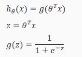
之前我们介绍过逻辑回归模型其函数值始终在0~1之间,因此我们给出其数学表达式为:hθ(x) = g(z),其中g代表逻辑函数(也称为S形函数),其表达式为:
其函数图为:
该数学表达式中的 z = θTX,其中X为特征向量。因此,我们可将表达式改写成:
关于逻辑函数hθ(x)的函数值我们可以理解为在自变量x和参数θ分别取得某个值的情况下y=0或者y=1的概率,即hθ(x) = P(y=0|x;θ)或者hθ(x) = P(y=1|x;θ)。
由于逻辑回归模型其值非1即0,我们可得如下表达式:
hθ(x) = P(y=0|x;θ) + hθ(x) = P(y=1|x;θ) = 1
因此,我们可以根据上述表达式在已知y=0(或y=1)的概率下,可求得y=1(或y=0)的概率。
补充笔记
Hypothesis Representation
We could approach the classification problem ignoring the fact that y is discrete-valued, and use our old linear regression algorithm to try to predict y given x. However, it is easy to construct examples where this method performs very poorly. Intuitively, it also doesn’t make sense for hθ(x) to take values larger than 1 or smaller than 0 when we know that y ∈ {0, 1}. To fix this, let’s change the form for our hypotheses hθ(x) to satisfy 0≤hθ(x)≤1. This is accomplished by plugging θTx into the Logistic Function.
Our new form uses the "Sigmoid Function," also called the "Logistic Function":
The following image shows us what the sigmoid function looks like:
The function g(z), shown here, maps any real number to the (0, 1) interval, making it useful for transforming an arbitrary-valued function into a function better suited for classification.
hθ(x) will give us the probability that our output is 1. For example, hθ(x)=0.7 gives us a probability of 70% that our output is 1. Our probability that our prediction is 0 is just the complement of our probability that it is 1 (e.g. if probability that it is 1 is 70%, then the probability that it is 0 is 30%).
边界判定(Decision Boundary)
逻辑函数的函数图像如下图所示:
从函数图中,我们可以得出如下结论:
- 当z≥0时,即θTX ≥0,则有g(z)≥0.5,我们可以预测y=1
- 当z≥0时,即θTX <0,则有g(z)<0.5,我们可以预测y=0
注:该结论为假设函数hθ(x)的属性,而非数据集的属性。
现假设hθ(x) = g(θ0 + θ1x1 + θ2x2),且设θ0 = -3,θ1 = 1,θ2 = 1。该假设函数hθ(x)拟合如图所示的数据集,我们通过上述的结论可知当θ0 + θ1x1 + θ2x2 ≥ 0时,即x1 + x2 ≥ 3时,我们可以预测y=1。当x1 + x2 = 3时为一条直线,因此我们可以在图中画出一条直线,这条直线我们称之为边界判断。
直线右侧部分我们可以将其划为y=1部分,左侧部分我们可以将其划为y=0部分。
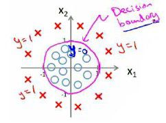
除此之外,若hθ(x) = g(θ0 + θ1x1 + θ2x2 + θ3x12 + θ4x22),设θ0 = -1,θ1 = 0,θ2 = 0,θ3 = 1,θ4 = 1,我们可以得到一个半径为1圆心在原点的圆,且拟合图中数据集。
我们也称这个圆为边界判定。通过这两个案例,我们可以知道边界判定可以是任何形状。
补充笔记
Decision Boundary
In order to get our discrete 0 or 1 classification, we can translate the output of the hypothesis function as follows:
The way our logistic function g behaves is that when its input is greater than or equal to zero, its output is greater than or equal to 0.5:
Remember.
So if our input to g is θTX, then that means:
From these statements we can now say:
The decision boundary is the line that separates the area where y = 0 and where y = 1. It is created by our hypothesis function.
Example:
In this case, our decision boundary is a straight vertical line placed on the graph where x1=5, and everything to the left of that denotes y = 1, while everything to the right denotes y = 0.
Again, the input to the sigmoid function g(z) (e.g. θTX) doesn't need to be linear, and could be a function that describes a circle (e.g. z=θ0+θ1x12+θ2x22) or any shape to fit our data.


