The method of sampling following the given distribution(invert cumulative distribution sampling)

In order to simulate a random variable X which follows a given distribution.

A direct approach to accomplish this task is a so-called invert cumulative distribution sampling.
This method can be applied in the scenario of the cumulative function is easy to derived when the distribution density function was provided.

The main steps of this approach:

1. derive the cumulative distribution function of the given distribution.

• derive the invert function of cumulative distribution function(CDF).
• generate a random variables which following uniform distribution.
• generate the result with this variable been substituted into CDF.
• Iterate step 1 to step 4 for sampling.

The result of step 4 is a sampled result which follows the given distribution.

By using R, we can process these steps easily with the provided functions.
We’d like to select beta distribution as an example.

In R, there are four functions related to the beta distribution: dbeta, pbeta, qbeta, rbeta.

dbeta gives the density, pbeta the distribution function, qbeta the quantile function, and rbeta generates random deviates.

dbeta: beta distribution function
pbeta: cumulative distribution function of beta distribution
qbeta: invert cumulative distribution function of beta distribution

We’ll employ qbeta in our case.
Besides, we also need a function called “runif” to generate random variable x within 0-1 which would be used as the parameters of invert CDF(qbeta at here).

In order to elaborate this method more intuitively, I'd like to use R to plot some example images.

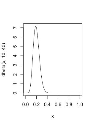
Suppose that we defined a beta distribution B(10,40).
We can draw the image of its distribution function by command in R:

curve (dbeta(x, 10, 40), xlim = c(0,1))

beta distribution density function of B(10,40)

Firstly, we generate a sequence variable from 0 to 1 with interval of 0.01 as x.

x = seq(0,1,0.01)

And then, the cumulative distribution function(CDF) of beta distribution could be paint like the image shows below:

![CDF of B(10,40]](http://upload-images.jianshu.io/upload_images/206991-7c1af38a74b9f4ca.png?imageMogr2/auto-orient/strip%7CimageView2/2/w/1240)

by the command in R:

curve (pbeta(x, 10, 40), xlim = c(0,1))

Besides, the invert CDF could be shown like this:

invert CDF of B(10,40)

by the command in R:

curve (qbeta(x, 10, 40), xlim = c(0,1))

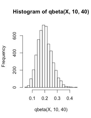
When x = 0.2, pbeta(x,10,40) equals 0.5282958. That means the probability of 0

We can locate this point by:

abline(h=qbeta(0.2,10,40), v=0.2, col = "red")

The point when x=0.2 on the CDF

The sampling would be proceed by repeat these steps above.

Finally, in order to verify the correctness of our method we can plot the histogram of a big amount of the sampling result. And it will show the difference between the original distribution and the results from sampling method.

For example，let's generate 5000 sampled value which following the given distribution beta(10,40) and plot the histogram of it.

X = runif(5000,min=0,max=1)
hist(qbeta(X,10,40),breaks = 20)

Histogram of the sampling results

The curve is similar with beta(10,40).