1.Perceptron
1.1 Description of Perceptron
Rosenblatt proposed the algorithm that would automatically learn the optimal weight coefficients that are then multiplied with the input features in order to make the decision of whether a neuron res or not.
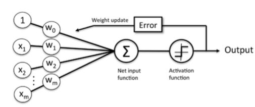
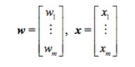
input feature: x=[x1,...,xm]
weight: w=[w1,...,wm]
More formally, we can pose this problem as a binary classification task where we refer to our two classes as 1 (positive class) and -1 (negative class) for simplicity. We
can then define an activation function φ(z) that takes a linear combination of certain
input values x and a corresponding weight vector w , where z is the so-called net
input ( z = w 1x 1+...+ w mx m ).
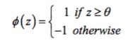
Now, if the activation of a particular sample x i,that is, the output of φ(z), is
greater than a de ned threshold θ , we predict class 1 and class -1, otherwise, in the
perceptron algorithm, the activation function φ (⋅) is a simple unit step function, which is sometimes also called the Heaviside step function:
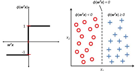
The following gure illustrates how the net input z = w Tx is squashed into a binary output (-1 or 1) by the activation function of the perceptron (left sub gure) and how it can be used to discriminate between two linearly separable classes (below):
Then using reductionist approach to mimic how a single neuron in the brain works: it either res or it doesn't. Thus, Rosenblatt's initial perceptron rule is fairly simple and can be summarized by the following steps:
- Initialize the weights to 0 or small random numbers.
- For each training sample x(i) perform the following steps:
- Compute the output value y^ .
- Update the weights.
Here, the output value is the class label predicted by the unit step function that we defined earlier, and the simultaneous update of each weight wj in the weight vector
w can be more formally written as:
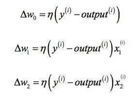
The value of ∆wj , which is used to update the weight w j , is calculated by the perceptron learning rule:
Where η is the learning rate (a constant between 0.0 and 1.0),
y (i) is the true class label of the i th training sample
y^ (i) is the predicted class label
It is important to
note that all weights in the weight vector are being updated simultaneously, which
means that we don't recompute the y^ (i) before all of the weights ∆w (j) were updated. Concretely, for a 2D dataset, we would write the update as follows:
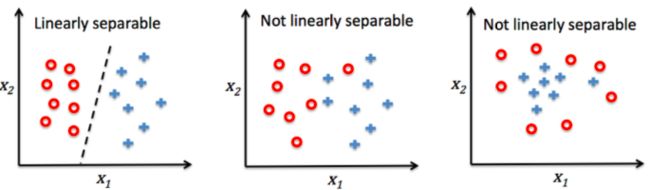
It is important to note that the convergence of the perceptron is only guaranteed if the two classes are linearly separable and the learning rate is suf ciently small. If the two classes can't be separated by a linear decision boundary, we can set a maximum number of passes over the training dataset (epochs) and/or a threshold for the number of tolerated misclassi cations—the perceptron would never stop updating the weights otherwise:
1.2 Implementing a perceptron learning algorithm in Python
First we will take an objected-oriented approach to de ne the perceptron interface as a Python Class, which allows us to initialize new perceptron objects that can learn from data via a fit method, and make predictions via a separate predict method. As a convention, we add an underscore to attributes that are not being created upon the initialization of the object but by calling the object's other methods—for example, self.w_.
#coding by my perceptron

import numpy as np

class Perceptron(object):
    """Perceptron classifier.

    Parameters
    ------------
    eta : float
        Learning rate (between 0.0 and 1.0)
    n_iter : int
        Passes over the training dataset.

    Attributes
    -----------
    w_ : 1d-array
        Weights after fitting.
    errors_ : list
        Number of misclassifications (updates) in each epoch.

    """
    def _init_(self,eta=0.01,n_iter=10):
        self.eta = eta
        self.n_iter = n_iter

    def fit(self, X, y):
        """Fit training data.

        Parameters
        ----------
        X : {array-like}, shape = [n_samples, n_features]
            Training vectors, where n_samples is the number of samples and
            n_features is the number of features.
        y : array-like, shape = [n_samples]
            Target values.

        Returns
        -------
        self : object

        """
        self.w_ = np.zeros(1 + X.shapes(1))
        self.errors_ = []
        for i in range(self.n_iter):
            errors = 0
            for Xi,target in zip(X,y):
                update = self.eta*(target - self.predict(Xi))
                self.w_[1:] += update*Xi
                self.w_[0] += update
                errors += int(update != 0.0)
            self.errors_.append(errors)
        return self


    def net_input(self, X):
        """Calculate net input"""
        return np.dot(X,self.w_[1:])+self.w_[0]


    def predict(self, X):
        """Return class label after unit step"""
        if self.net_input(X)>=0:
            return 1
        else:
            return -1
Using this perceptron implementation,we can now initialize new Perceptron objects with a given learning rate eta and n_iter, which is the number of epochs (passes over the training set). Via the fit method we initialize the weights in
self.w_ to a zero-vector R m+1 where m stands for the number of dimensions (features) in the dataset where we add 1 for the zero-weight (that is, the threshold).
After the weights have been initialized, the fit method loops over all individual samples in the training set and updates the weights according to the perceptron learning rule that we discussed in the previous section. The class labels are predicted by the predict method, which is also called in the fit method to predict the class label for the weight update, but predict can also be used to predict the class labels of new data after we have fitted our model. Furthermore, we also collect the number of misclassi cations during each epoch in the list self.errors_ so that we can
later analyze how well our perceptron performed during the training. The np.dot function that is used in the net_input method simply calculates the vector dot product wT x .
1.3 Training a perceptron model on the Iris dataset
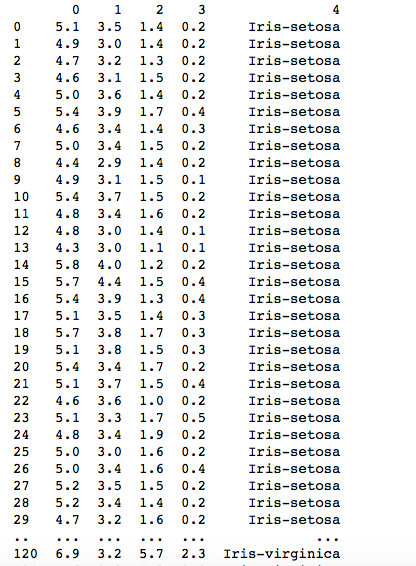
To test our perceptron implementation, we will load the two ower classes Setosa and Versicolor from the Iris dataset.
First,we will use the pandas library to load the Iris dataset directly from the UCI Machine Learning Repository into a DataFrame object and print the last ve lines via the tail method to check that the data was loaded correctly:
import pandas as pd

df = pd.read_csv('https://archive.ics.uci.edu/ml/machine-learning-databases/iris/iris.data', header=None)
df.head()
from matplotlib import pyplot as plt
import numpy as np

print df
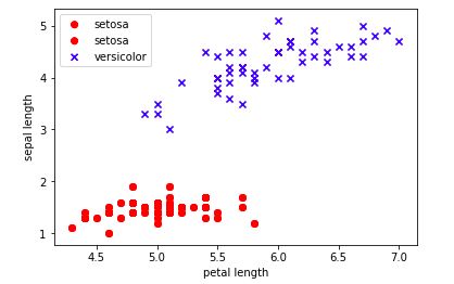
Next, we extract the rst 100 class labels that correspond to the 50 Iris-Setosa and 50 Iris-Versicolor owers, respectively, and convert the class labels into the two integer class labels 1 (Versicolor) and -1 (Setosa) that we assign to a vector y where the values method of a pandas DataFrame yields the corresponding NumPy representation. Similarly, we extract the rst feature column (sepal length) and the third feature column (petal length) of those 100 training samples and assign them to a feature matrix X, which we can visualize via a two-dimensional scatter plot:
y = df.iloc[0:100, 4].values
y = np.where(y == 'Iris-setosa', -1, 1)
X = df.iloc[0:100, [0, 2]].values

plt.scatter(X[:50, 0], X[:50, 1],color='red', marker='o', label='setosa')
plt.scatter(X[50:100, 0], X[50:100, 1],color='blue', marker='x', label='versicolor')
plt.xlabel('petal length')
plt.ylabel('sepal length')
plt.legend(loc='upper left')
plt.show()
Then we will train our perceptron algorithm on the Iris data subset that we just extracted.
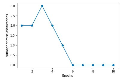
Also, we will plot the misclassification error for each epoch to check if the algorithm converged and found a decision boundary that separates the two Iris ower classes:
ppn = Perceptron(eta=0.1, n_iter=10)
ppn.fit(X, y)
plt.plot(range(1, len(ppn.errors_) + 1), ppn.errors_,marker='o')
plt.xlabel('Epochs')
plt.ylabel('Number of misclassifications')
plt.show()
As we can see in the preceding plot, our perceptron already converged after the sixth epoch and should now be able to classify the training samples perfectly. Let us implement a small convenience function to visualize the decision boundaries for 2D datasets:
from matplotlib.colors import ListedColormap


def plot_decision_regions(X, y, classifier, resolution=0.02):

    # setup marker generator and color map
    markers = ('s', 'x', 'o', '^', 'v')
    colors = ('red', 'blue', 'lightgreen', 'gray', 'cyan')
    cmap = ListedColormap(colors[:len(np.unique(y))])

    # plot the decision surface
    x1_min, x1_max = X[:, 0].min() - 1, X[:, 0].max() + 1
    x2_min, x2_max = X[:, 1].min() - 1, X[:, 1].max() + 1
    xx1, xx2 = np.meshgrid(np.arange(x1_min, x1_max, resolution),
                           np.arange(x2_min, x2_max, resolution))
    Z = classifier.predict(np.array([xx1.ravel(), xx2.ravel()]).T)
    Z = Z.reshape(xx1.shape)
    plt.contourf(xx1, xx2, Z, alpha=0.4, cmap=cmap)
    plt.xlim(xx1.min(), xx1.max())
    plt.ylim(xx2.min(), xx2.max())

    # plot class samples
    for idx, cl in enumerate(np.unique(y)):
        plt.scatter(x=X[y == cl, 0], y=X[y == cl, 1],
                    alpha=0.8, c=cmap(idx),
                    marker=markers[idx], label=cl)
First, we define a number of colors and markers and create a color map from
the list of colors via ListedColormap.
Then, we determine the minimum and maximum values for the two features and use those feature vectors to create a pair of grid arrays xx1 and xx2 via the NumPy meshgrid function.
Since we trained our perceptron classi er on two feature dimensions, we need to atten the grid arrays and create a matrix that has the same number of columns as the Iris training subset so that we can use the predict method to predict the class labels Z of the corresponding grid points.
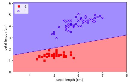
After reshaping the predicted class labels Z into a grid with the same dimensions as xx1 and xx2, we can now draw a contour plot via matplotlib's contourf function that maps the different decision regions to different colors for each predicted class in the grid array:
plot_decision_regions(X, y, classifier=ppn)
plt.xlabel('sepal length [cm]')
plt.ylabel('petal length [cm]')
plt.legend(loc='upper left')

plt.tight_layout()
# plt.savefig('./perceptron_2.png', dpi=300)
plt.show()
2.Adaptive linear neurons and the convergence of learning
2.1 Description of Adaline(Adaptive Linear Neuron )
It is another type of single-layer neural network,and can be considered as an improvement on the latter.
The key difference between the Adaline rule (also known as the Widrow-Hoff rule) and Rosenblatt's perceptron is that the weights are updated based on a linear activation function rather than a unit step function like in the perceptron. In Adaline,
this linear activation function φ(z) is simply the identity function of the net input so that φ(wT x)=wTx.
While the linear activation function is used for learning the weights, a quantizer, which is similar to the unit step function that we have seen before, can then be used to predict the class labels, as illustrated in the following gure:
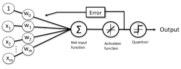
If we compare the preceding gure to the illustration of the perceptron algorithm that we saw earlier, the difference is that we know to use the continuous valued output from the linear activation function to compute the model error and update the weights, rather than the binary class labels.
Minimizing cost functions with gradient descent
One of the key ingredients of supervised machine learning algorithms is to define an objective function that is to be optimized during the learning process. This objective function is often a cost function that we want to minimize. In the case of Adaline, we can define the cost function J to learn the weights as the Sum of
Squared Errors (SSE) between the calculated outcome and the true class label:
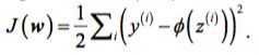
The main advantage of this continuous linear activation function is—in contrast to the unit step function—that the cost function becomes differentiable. Another nice property of this cost function is that it is convex; thus, we can use a simple, yet powerful, optimization algorithm called gradient descent to nd the weights that minimize our cost function to classify the samples in the Iris dataset.
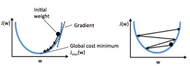
As illustrated in the following gure, we can describe the principle behind gradient descent as climbing down a hill until a local or global cost minimum is reached. In each iteration, we take a step away from the gradient where the step size is determined by the value of the learning rate as well as the slope of the gradient:
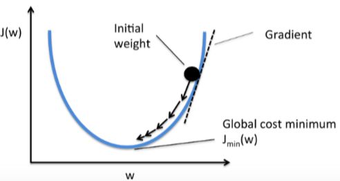
Using gradient descent, we can now update the weights by taking a step away from the gradient ∇J(w) of our cost function J(w):
w := w + ∆w
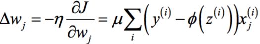
Here, the weight change ∆w is de ned as the negative gradient multiplied by the
learning rate η :
∆w = −η∆J(w).
To compute the gradient of the cost function, we need to compute the partial derivative of the cost function with respect to each weight
derivative of the cost function with respect to each weight:
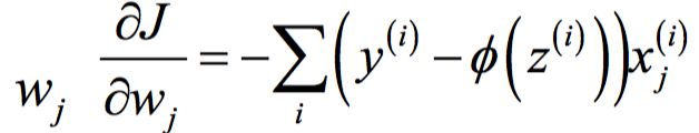
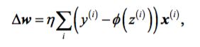
so that we can write the update of weight w j as:
Since we update all weights simultaneously, our Adaline learning rule becomes
w := w + ∆w
2.1 Implemention
Since perceptron rule and Adaline are very similar ,we will take the perceptron implementation that we defined earlier and change the fit method so that the weights are updated by minimizing the cost function via gradient descent.
#coding by my perceptron

import numpy as np

class Myperceptron(object):
    """Perceptron classifier.

    Parameters
    ------------
    eta : float
        Learning rate (between 0.0 and 1.0)
    n_iter : int
        Passes over the training dataset.

    Attributes
    -----------
    w_ : 1d-array
        Weights after fitting.
    errors_ : list
        Number of misclassifications (updates) in each epoch.

    """
    def __init__(self, eta,n_iter):
        self.eta = eta
        self.n_iter = n_iter

    def fit(self, X, y):
        """Fit training data.

        Parameters
        ----------
        X : {array-like}, shape = [n_samples, n_features]
            Training vectors, where n_samples is the number of samples and
            n_features is the number of features.
        y : array-like, shape = [n_samples]
            Target values.

        Returns
        -------
        self : object

        """
        self.w_ = np.zeros(1 + X.shape[1])
        self.errors_ = []
        for i in range(self.n_iter):
            errors = 0
            for Xi,target in zip(X,y):
                update = self.eta*(target - self.predict(Xi))
                self.w_[1:] += update*Xi
                self.w_[0] += update
                errors += int(update != 0.0)
            self.errors_.append(errors)
        return self


    def net_input(self, X):
        """Calculate net input"""
        return np.dot(X,self.w_[1:])+self.w_[0]


    def predict(self, X):
        """Return class label after unit step"""
        if self.net_input(X)>=0:
            return 1
        else:
            return -1
Instead of updating the weights after evaluating each individual training sample, as in the perceptron, we calculate the gradient based on the whole training dataset via self.eta * errors.sum() for the zero-weight and via self.eta * X.T.dot(errors) for the weights 1 to m where X.T.dot(errors) is a matrix-vector multiplication between our feature matrix and the error vector. Similar to the previous perceptron implementation, we collect the cost values in a list self.cost_ to check if the algorithm converged after training.
In practice, it often requires some experimentation to nd a good learning rate η for optimal convergence. So, let's choose two different learning rates η = 0.1 and η = 0.0001 to start with and plot the cost functions versus the number of epochs to see how well the Adaline implementation learns from the training data.
Let us now plot the cost against the number of epochs for the two different learning rates:
df = pd.read_csv('https://archive.ics.uci.edu/ml/machine-learning-databases/iris/iris.data', header=None)
df.head()


y = df.iloc[0:100, 4].values
y = np.where(y == 'Iris-setosa', -1, 1)
X = df.iloc[0:100, [0, 2]].values

fig, ax = plt.subplots(nrows=1, ncols=2, figsize=(8, 4))


ada1 = my_AdalineGD(n_iter=10, eta=0.01).fit(X, y)
ax[0].plot(range(1, len(ada1.cost_) + 1), np.log10(ada1.cost_), marker='o')
ax[0].set_xlabel('Epochs')
ax[0].set_ylabel('log(Sum-squared-error)')
ax[0].set_title('Adaline - Learning rate 0.01')

ada2 = AdalineGD(n_iter=10, eta=0.0001).fit(X, y)
ax[1].plot(range(1, len(ada2.cost_) + 1), ada2.cost_, marker='o')
ax[1].set_xlabel('Epochs')
ax[1].set_ylabel('Sum-squared-error')
ax[1].set_title('Adaline - Learning rate 0.0001')

plt.tight_layout()
plt.savefig('./adaline_1.png', dpi=300)
plt.show()
As we can see in the resulting cost function plots next, we encountered two different types of problems. The left chart shows what could happen if we choose a learning rate that is too large—instead of minimizing the cost function, the error becomes larger in every epoch because we overshoot the global minimum:
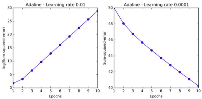
We need to choice a suitable learning rate.If the value is too small,that the algorithm need a number of epochs .If the value is too big,it will overshoot the global minimum. About these situation,we can see the plot below.
standardization:it´s a kind of feature scaling,which gives our data the property of a standard normal distribution.
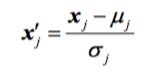
While U j is samples mean value and σ j standard deviation(标准差in python,we use .std()).
X_std = np.copy(X)
X_std[:,0] = (X[:,0]-X[:,0].mean()) / X[:,0].std()
X_std[:,1] = (X[:,1]-X[:,1].mean()) / X[:,1].std()
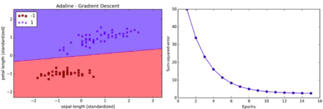
After standardization, we will train the Adaline again and see that it now converges using a learning rate η = 0.01:
ada = AdalineGD(n_iter=15, eta=0.01)
ada.fit(X_std, y)

plot_decision_regions(X_std, y, classifier=ada)
plt.title('Adaline - Gradient Descent')
plt.xlabel('sepal length [standardized]')
plt.ylabel('petal length [standardized]')
plt.legend(loc='upper left')
plt.tight_layout()
# plt.savefig('./adaline_2.png', dpi=300)
plt.show()

plt.plot(range(1, len(ada.cost_) + 1), ada.cost_, marker='o')
plt.xlabel('Epochs')
plt.ylabel('Sum-squared-error')

plt.tight_layout()
# plt.savefig('./adaline_3.png', dpi=300)
plt.show()
Large scale machine learning
A popular alternative to the batch gradient descent algorithm is stochastic gradient descent, sometimes also called iterative or on-line gradient descent. Instead of updating
the weights based on the sum of the accumulated errors over all samples x(i) :
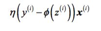
We update the weights incrementally for each training sample:
and stochastic gradient descent can be considered as an approximation of gradient descent, it typically reaches convergence much faster because of the more frequent weight updates. Since each gradient is calculated based on a single training example, the error surface is noisier than in gradient descent, which can also have the advantage that stochastic gradient descent can escape shallow local minima more readily. To obtain accurate results via stochastic gradient descent, it is important to present it with data in a random order, which is why we want to shuffle the training set for every epoch to prevent cycles.
import numpy as np
from numpy.random import seed

class my_AdalineSGD(object):
    def __init__(self, eta=0.01, n_iter=10, shuffle=True, random_state=None):
        self.eta = eta
        self.n_iter = n_iter
        self.w_initialized = False
        self.shuffle = shuffle
        if random_state:
            seed(random_state)

    def _shuffle(self,X,y):
        r = np.random.permutation(len(y))
        return X[r],y[r]

    def _initial_weight(self,m):
        self._w = np.zeros(m + 1)
        self.w_initialized = True

    def net_input(self,X):
        return np.dot(X,self._w[1:])+self._w[0]

    def activation(self,X):
        return self.net_input(X)

    def predict(self,X):
        return np.where(self.activation(X)>=0.0,1,-1)

    def _update_weight(self,xi,target):
        output = self.net_input(xi)
        error = (target-output)
        self._w[1:] += self.eta * xi.dot(error)
        self._w[0] += self.eta*error
        cost = 0.5 * error**2
        return cost

    def fit(self,X,y):
        self._initial_weight(X.shape[1])
        self.cost_ = []
        for i in range(self.n_iter):
            if self.shuffle
                X,y = self._shuffle(X,y)
            cost = []
            for xi,target in zip(X,y):
                cost.append(self._update_weight(xi,target))
            avg_cost = sum(cost)/len(y)
            self.cost_.append(avg_cost)
        return self

    def partial_fit(self, X, y):
        """Fit training data without reinitializing the weights"""
        if not self.w_initialized:
            self. _initial_weight(X.shape[1])
        if y.ravel().shape[0] > 1:
            for xi, target in zip(X, y):
                self._update_weight(xi, target)
        else:
            self._update_weight(X, y)
        return self
plot the figure
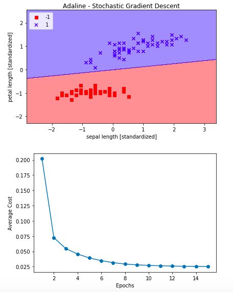
ada = my_AdalineSGD(n_iter=15, eta=0.01, random_state=1)
ada.fit(X_std, y)

plot_decision_regions(X_std, y, classifier=ada)
plt.title('Adaline - Stochastic Gradient Descent')
plt.xlabel('sepal length [standardized]')
plt.ylabel('petal length [standardized]')
plt.legend(loc='upper left')

plt.tight_layout()
#plt.savefig('./adaline_4.png', dpi=300)
plt.show()

plt.plot(range(1, len(ada.cost_) + 1), ada.cost_, marker='o')
plt.xlabel('Epochs')
plt.ylabel('Average Cost')

plt.tight_layout()
# plt.savefig('./adaline_5.png', dpi=300)
plt.show()
Summary
In this chapter, we gained a good understanding of the basic concepts of linear classi ers for supervised learning. After we implemented a perceptron, we saw how we can train adaptive linear neurons ef ciently via a vectorized implementation
of gradient descent and on-line learning via stochastic gradient descent. Now that we have seen how to implement simple classi ers in Python, we are ready to move on to the next chapter where we will use the Python scikit-learn machine learning library to get access to more advanced and powerful off-the-shelf machine learning classi ers that are commonly used in academia as well as in industry.