对于不同数据集合的比较的可视化,一般用韦恩图来表示,但是数据集合太多了,就不好看了,反而不容易从图中获得信息了。
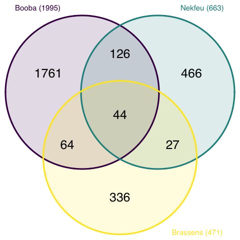
三个集合看起来最合适。
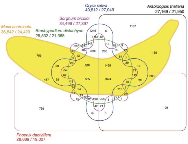
香蕉基因组
2012年发表的香蕉基因组文章中的韦恩图,已经很美观了,但阅读起来还是比较费劲的。
为了解决过多的数据集合造成的信息混乱问题,UpsetR包应运而生完美解决了这个问题,这个包的使用教程网上也比较多。
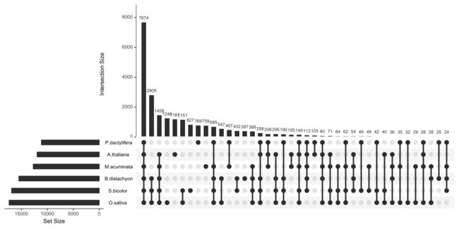
今天看见Y叔推荐了ggplot2风格的upset plot——ggupset包,顺便学习一下这个包的使用教程,我这个有点跟风的嫌疑,感谢Y叔的分享。
1.安装ggupset
# Download package from CRAN
> install.packages("ggupset")

# Or get the latest version directly from GitHub
> devtools::install_github("const-ae/ggupset")
2.示例
> library(ggplot2)
> library(tidyverse)
> library(ggupset)
#使用的数据集tidy_movies,IMDB中的电影列表
> tidy_movies
# A tibble: 50,000 x 10
   title                                    year length  budget rating votes mpaa  Genres    stars percent_rating

 1 Ei ist eine geschissene Gottesgabe, Das  1993     90      NA    8.4    15 ""         1            4.5
 2 Hamos sto aigaio                         1985    109      NA    5.5    14 ""         1            4.5
 3 Mind Benders, The                        1963     99      NA    6.4    54 ""         1            0
 4 Trop (peu) d'amour                       1998    119      NA    4.5    20 ""         1           24.5
 5 Crystania no densetsu                    1995     85      NA    6.1    25 ""         1            0
 6 Totale!, La                              1991    102      NA    6.3   210 ""         1            4.5
 7 Visiblement je vous aime                 1995    100      NA    4.6     7 ""         1           24.5
 8 Pang shen feng                           1976     85      NA    7.4     8 ""         1            0
 9 Not as a Stranger                        1955    135 2000000    6.6   223 ""         1            4.5
10 Autobiographia Dimionit                  1994     87      NA    7.4     5 ""         1            0
# ... with 49,990 more rows
> > tidy_movies %>%
+     distinct(title, year, length, .keep_all=TRUE) %>%
+     ggplot(aes(x=Genres)) +
+     geom_bar() +
+     scale_x_upset(n_intersections = 20)
Warning message:
Removed 100 rows containing non-finite values (stat_count).
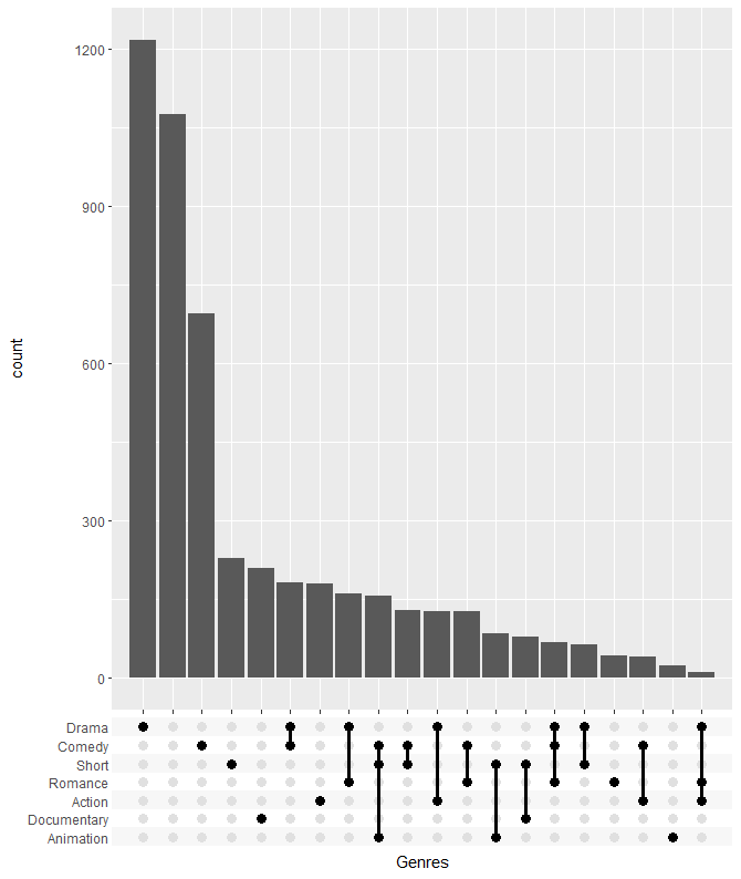 不同类型的电影
不同类型的电影
查看更细致的电影分类情况
> tidy_movies %>%
+     distinct(title, year, length, .keep_all=TRUE) %>%
+     mutate(Genres_collapsed = sapply(Genres, function(x) paste0(sort(x), collapse = "-"))) %>%
+     select(title, Genres, Genres_collapsed)
# A tibble: 5,000 x 3
   title                                   Genres    Genres_collapsed

 1 Ei ist eine geschissene Gottesgabe, Das  Documentary
 2 Hamos sto aigaio                         Comedy
 3 Mind Benders, The                        ""
 4 Trop (peu) d'amour                       ""
 5 Crystania no densetsu                    Animation
 6 Totale!, La                              Comedy
 7 Visiblement je vous aime                 ""
 8 Pang shen feng                           Action-Animation
 9 Not as a Stranger                        Drama
10 Autobiographia Dimionit                  Drama
# ... with 4,990 more rows
> tidy_movies %>%
+     distinct(title, year, length, .keep_all=TRUE) %>%
+     mutate(Genres_collapsed = sapply(Genres, function(x) paste0(sort(x), collapse = "-"))) %>%
+     ggplot(aes(x=Genres_collapsed)) +
+     geom_bar() +
+     theme(axis.text.x = element_text(angle=90, hjust=1, vjust=0.5))
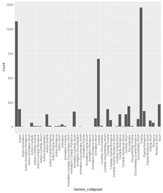 细分的电影类型
细分的电影类型
根据上述结果,生成新的电影分类方式。
> tidy_movies %>%
+     distinct(title, year, length, .keep_all=TRUE) %>%
+     ggplot(aes(x=Genres)) +
+     geom_bar() +
+     scale_x_mergelist(sep = "-") +
+     theme(axis.text.x = element_text(angle=90, hjust=1, vjust=0.5))
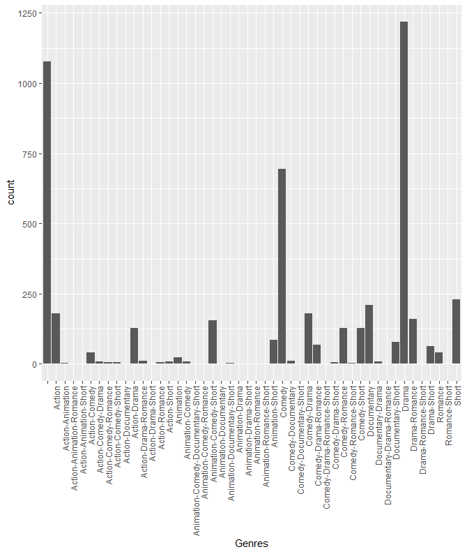 新的电影分类
新的电影分类
展示不同类型电影之间的关系
> tidy_movies %>%
+     distinct(title, year, length, .keep_all=TRUE) %>%
+     ggplot(aes(x=Genres)) +
+     geom_bar() +
+     scale_x_mergelist(sep = "-") +
+     axis_combmatrix(sep = "-")
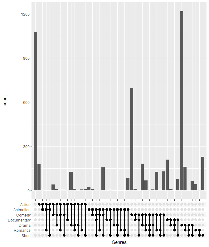 不同类型电影之间的关系
不同类型电影之间的关系
不同的图形类型
每种类型电影的总数量
> tidy_movies %>%
+     distinct(title, year, length, .keep_all=TRUE) %>%
+     unnest() %>%
+     mutate(GenreMember=1) %>%
+     spread(Genres, GenreMember, fill=0) %>%
+     as.data.frame() %>%
+     UpSetR::upset(sets = c("Action", "Romance", "Short", "Comedy", "Drama"), keep.order = TRUE)

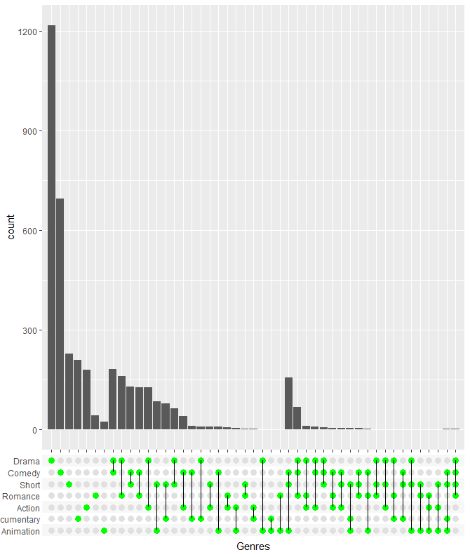
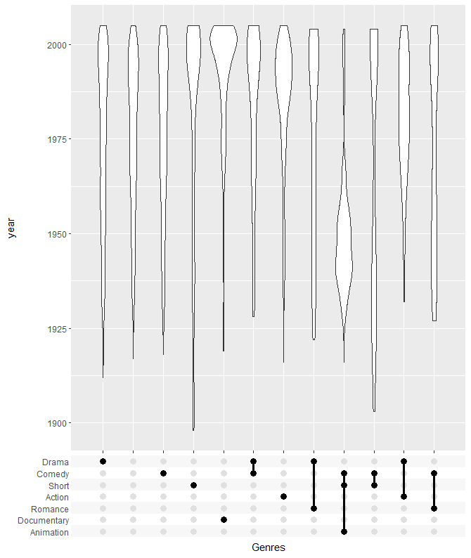
使用小提琴图展示
> tidy_movies %>%
+     distinct(title, year, length, .keep_all=TRUE) %>%
+     ggplot(aes(x=Genres, y=year)) +
+     geom_violin() +
+     scale_x_upset(order_by = "freq", n_intersections = 12)
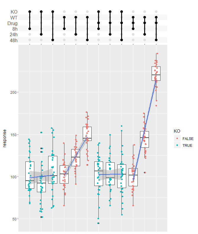
3.更出色的范例
使用箱线图,散点图和拟合曲线展示结果
> df_complex_conditions
# A tibble: 360 x 4
   KO    DrugA Timepoint response

 1 TRUE  Yes           8     84.3
 2 TRUE  Yes           8    105.
 3 TRUE  Yes           8     79.1
 4 TRUE  Yes           8    140.
 5 TRUE  Yes           8    108.
 6 TRUE  Yes           8     79.5
 7 TRUE  Yes           8    112.
 8 TRUE  Yes           8    118.
 9 TRUE  Yes           8    114.
10 TRUE  Yes           8     92.4
# ... with 350 more rows
> df_complex_conditions %>%
+     mutate(Label = pmap(list(KO, DrugA, Timepoint), function(KO, DrugA, Timepoint){
+         c(if(KO) "KO" else "WT", if(DrugA == "Yes") "Drug", paste0(Timepoint, "h"))
+     })) %>%
+     ggplot(aes(x=Label, y=response)) +
+     geom_boxplot() +
+     geom_jitter(aes(color=KO), width=0.1) +
+     geom_smooth(method = "lm", aes(group = paste0(KO, "-", DrugA))) +
+     scale_x_upset(order_by = "degree",
+                   sets = c("KO", "WT", "Drug", "8h", "24h", "48h"),
+                   position="top", name = "") +
+     theme_combmatrix(combmatrix.label.text = element_text(size=12),
+                      combmatrix.label.extra_spacing = 5)
不同类型电影的IMDBD评分情况
> avg_rating <- tidy_movies %>%
+     mutate(Genres_collapsed = sapply(Genres, function(x) paste0(sort(x), collapse="-"))) %>%
+     mutate(Genres_collapsed = fct_lump(fct_infreq(as.factor(Genres_collapsed)), n=12)) %>%
+     group_by(stars, Genres_collapsed) %>%
+     summarize(percent_rating = sum(votes * percent_rating)) %>%
+     group_by(Genres_collapsed) %>%
+     mutate(percent_rating = percent_rating / sum(percent_rating)) %>%
+     arrange(Genres_collapsed)
> avg_rating
# A tibble: 130 x 3
# Groups:   Genres_collapsed [13]
   stars Genres_collapsed percent_rating

 1     1 Drama                    0.0437
 2     2 Drama                    0.0411
 3     3 Drama                    0.0414
 4     4 Drama                    0.0433
 5     5 Drama                    0.0506
 6     6 Drama                    0.0717
 7     7 Drama                    0.129
 8     8 Drama                    0.175
 9     9 Drama                    0.170
10    10 Drama                    0.235
# ... with 120 more rows

# Plot using the combination matrix axis
# the red lines indicate the average rating per genre
> ggplot(avg_rating, aes(x=Genres_collapsed, y=stars, fill=percent_rating)) +
+     geom_tile() +
+     stat_summary_bin(aes(y=percent_rating * stars), fun.y = sum,  geom="point",
+                      shape="—", color="red", size=6) +
+     axis_combmatrix(sep = "-", levels = c("Drama", "Comedy", "Short",
+                                           "Documentary", "Action", "Romance", "Animation", "Other")) +
+     scale_fill_viridis_c()
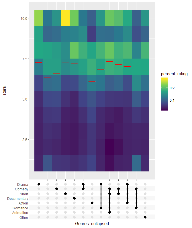
不同类型电影的IMDBD评分
粗略的走了一遍教程,结束!