Introduction to Statistical Mechanics, Phase Transitions, and the Ising Model

• Name: 贺一珺
• Student Number: 2014302290002
• Class: 物理学弘毅班

Abstract

In statistical physics, we are interested in multi-particle and many-state systems particularly where the interactions between particles play an essntial role, which can exhibit a phenomenon known as a phase transition. This phenomenon can be observed universally in nature such as the appearance of ferromagnetism in materials such as iron. The transition like this require the concept of temperature, which is quite significant in condensed matter physics.
In this article I will give a brief introduction to Ising model and try to use it to investigate several properties of solid like Magnetization, Energy per spin, Specific heat per spin and susceptibility of particles. To do all of these works, I will use Mean Field Theory which is widely used in the study of statistical mechanics to symplify the calculation and use the Monte Carco Method which is useful when solving some numerical problems to simulate the process of thermalequibulum in real world. What's more, phase transitions will also be investigated in this article so that one could have a deeper understanding about the equilibrium state under various tempreture and appreciate the tremendous beauty of the real world.
All of my codes are uploaded here

Background

Ising Model

Magnetism is an inherently quantum phenomena which cannot be exhibited classically. To decribe the behavior of a magnetic material, we should introduce the electron's spin and the associated magnetic moment in quantum mechanics. The Ising model is a mathematical model of ferromagnetism in statistical mechanics. In Ising Model, the spins are arranged in a graph, usually a lattice, allowing each spin to interact with its neighbors. Ferromagnetism arises when a collection of such spins conspire so that all of their magnetic moments point in the same direction, yielding a total moment that is macroscopic in size. Each spin is able to point at two directions and thus can be denoted by two numbers. After we introduce the concept of spin, the energy of the system is given by these neighbouring interactions and the interaction between the spins and an external magnetic field:

Energy

For simplicity, we assume that:

.
for neighberhood spins.
Less energy is prefered by a system, thus it can be derived that for a ferromagnetic material all spin are aligned.
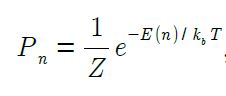
Assuming that our spin system is in equilibrium with a heat bath at temperature T, so that we can use the conclusion of statistical mechanics directly. The probability of finding the system in any particular state is proportional to the Boltzmann factor

Boltzmann Distribution

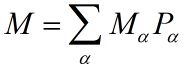
And then we get the measured magnetization of the system:

Magnetization

where

Ising quench(From wikipedia)

Mean Field Theory

Mean field theory is a useful approach for calculating the properties of a spin system. The magnetization is related to the average spin alignment. For an infinitely large system, the spins will all have the same average alignment.Hence all spins must have the same average properties. The total magnetization at temprature T for a system of N spins will then be

Total Magnetization

Thus we can derive M if we can calculate . An exact computation of would require the probabilities of all possible microstates. We cannot do this completely constricted by our ability to calculate. The only thing we can do is to consider an approximate alternative known as mean field theory.
Using the result of statistical mechanics, the thermal average of si can be calculated as

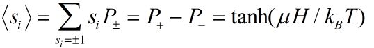
This is the exact result for the behavior of a single spin in a magnetic field. Now consider an approximate method: The interaction of a spin with its neighbering spins is equivalent to an effective magnetic field acting on si.So the thing we need to do first is to calculate the effective field Heff.
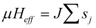
The energy function can be rewritten in this form:

Total Energy

which shows that the term involving J has the form of a magnetic field with

Then we have the following relationship

and

The Monte Carlo Method

The mean field theory we mensioned before is not always valid. A critical example is the values of the critical exponent. A more powerful approach is the Monte Carlo Method.

Rayleigh Taylor instability(From Wikipedia)

To simulate how a spin system interacts with its environment, we will consider the particular case of a collection of Ising spins. The Monte Carlo method uses a stochastic approach to simulate the exchange of energy between the spin system and the heat bath. A spin is chosen and the energy required to make it flip is calculated. If Eflip is negative, the spin is flipped and the system moves into a different microstate. If Eflip is positive, a decision must be made. The core of the Monte Carlo method is to use the computer to generate some randon numbers which satisfy the Boltzmann distribution. The approach to realize this is to compare the numbergenerated with the function derived from the Boltzmann factos which we mensioned before.

Realization of progrem

I use more than 10 progrem to finish this article and I will describe some of them so that readers could have a deeper understanding about the theory I mensioned before.
All of my codes are uploaded here

• Getting the solution of the equation of
  1. A direct method to do this is to plot both the right side and the left side of the equation in one picture. The solution is the x axis of their cross point. I take J=4 here for two dimensional cases. Temperature and volue of z can be modefied directly before we runthe progrem as the initial condition.

  2. Also, we can use the Newton-Raphson method to get the solusion which is useful when soving many equation. But this method requires a good property of converience. And sometimes this method is pretty relay on the choice of initial conditions. 
     

• Ising Model using the Monte Carlo Method
  1. First I creat the function to generate the matrex and random number automatedly.
  2. Each site in the matrex will have some contribution to the total energy. I define the function to calculate this by adding up the energy generated by the interaction of spin and field of the four sites near the point.
  3. Define the function to calculate the total energy by simply adding up the energy of all points in the matrix.
  4. Calculate the Eflip. Note that it can be expressed as the difference of the energy of two spin in the same site.
  5. In this step I will try to use the Metropolis algorithm. This is the most crutial and difficult part in this progrem.

  - Firstly I tried to simply calculate the flip energy in each site of the matrix and generate the random number to do the Monte Carlo process in order to renew the states of the whole matrix, but I found that the value generated by the progrem is not random as I expected. Here I show my code: ##
  

  • Then I tried to improve my progrem to solve this problem, what I did is to consider the concept of equabulium. I choose the site randomly until the progrem run about 100000 times to garentee that each site is equally considered. Then I use 'if' paragraph to decide weather the system is in equalibrium or not. This time the problem is solved.
  • To see the details, please see the progrem I uploaded on Github.

Results

All of my codes are uploaded here

The Ising Model, Statistical Mechanics and Mean Field Theory

The first method to work out the equation

Using the cross point to work out the equation

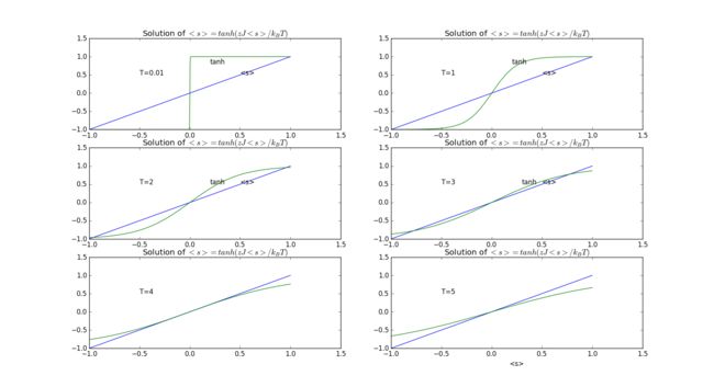
• Here is the two side of equation under various tempreture. It can be derived from the picture that Tc=4 is the critical temperature which denote the temperature when phase transition occurs.

Solve the equation using the Newton-Raphson method

Newton-Raphson method

• When using the Newton-Raphson method, one expect the curve to converge to a fixed volue. Here I calculated the cases of T=1, 2, 3. One can see from picyure that when calculate the solution when T=3, the method is not converge.

Here I zoomed the curve so that readers could read more clearly:

• It can be concluded that when T=1, the average spin approximates 0.9993;
• When T=2, the average spin approximates 0.9575;
• When T=3, the curve does not converge.

The method takes only about 3 steps to reach the result. Thus this is an effective method when calculate the solution.

To investigate the property of average spin near transition point T=4, I calculated the equation when T=3.9. Here is the result:

Solution of equation when T=3.9

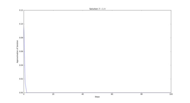
• It can be concluded that the result is very close to 0.

Further more, I tried to reset the initial condition when T=1 and look whether it converges:

Different initial condition when T=1

The Monte Carlo Method, Ising Model and Second-Order Phase Transition

Magnetization versus time under T=1, 2, 3,... ,6

I plotted the curves of magnetization versus time(Loop) under different temperature:

Magnetization versus time

• Different color stands for different temperature. One can see directly that as time increase the magnetization changes from 1 to 0 roughly, and when T=3 its range is largest.

Magnetization versus temperature

Magnetization

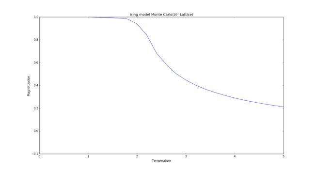
• In this picture we can see that when T is close to 2.2, the magnetization decrease repidly.
• I expect the curve to be close to 0 when tempreture is high and close to 1 when temperature is low. But the picture does not give the full information. I extended the range and did it again:

Magnetization

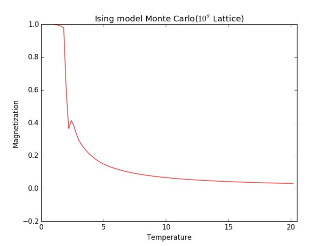
Here you can see that it satisfies our expectation! Note that the curve has a slope near the temperature 2.25. It stands for the phase transition.

Energy per spin versus tempreture

Energy per spin

• I calculated the energy per spin versus temperature. You can see from the picture that it is close to -2.0 when temperature is close to 1, and it goes close to -0.4 when temperature is close to 5.

Specific heat per spin

Specific heat per spin(Dots)

• Here I plotted the specific heat per spin using points. One can see that it has a shape of bell. When T is close to 2.25 it reaches its maximium.

• To explicit the tendency, I plotted a curve:

Specific heat versus time

Notice that the curve is not so stable near its maximium. It may because it varies too fast near it. Here I show you a more mussy one:

Then it can be easily seen that the points near the transition point T=2.25 is very mussy actually because of the large slope.

Susceptibility

Susceptibility versus temperature

• Here is the dots of suscptibility versus temperature. One can see that it remains 0 until temperature reaches 2 and suddenly it increase to 0.1. Approximately after T=3 it decrease and reaches a fixed volue slowly.

Here I plot the curve:

Susceptibility versus temperature(Curve)

States of lattice

At the end, I will show you the states of lattice under various temperature. These picture will give you a direct image:

Lattice

• White color stands for the spin up and black color stands for the spin down. The color of frame each lattice stands for different temperature.
• You can conclude from the picture that the entrepy increases as the temperature increases.
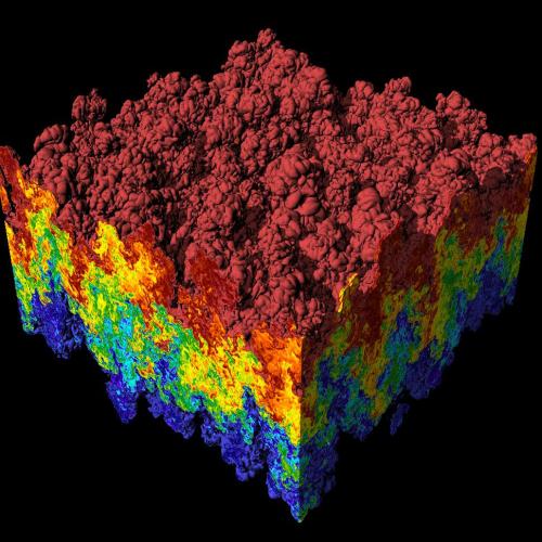
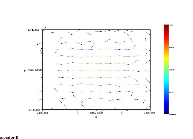
• Situations are more stimulating and complicated in 3-dimensional cases. Here I will show you a picture to lead you in to the amazing 3-dimensional world. (This picture is plotted using FDTD Solutions)

Acknowladgement

• Prof. Cai
• Computation physics