Deep Learning | 2 Improving Deep Neural Networks: Hyperparameter tuning, Regularization and Optimization

0 Intrduction

Best thanks to Professor Andrew Ng and his learning materials for deep learning. This note is based on the videos of Andrew Ng.

If you are a deep learning starter, I strongly recommend you to watch these videos, they are easy to understand, and totally free.

The rest part of this note is a brief summary of the materials, take a look if you like.

1 Setting Up Your ML Application

1.1 Train/Dev/Test Sets

---

Data = Training set + Hold-out Cross Validation Set / Development Set + Test Set

Workflow

• Training Set: Keep on training algorithm on your training set

• Dev Set: Use your dev set to see which of many different models perform best on your dev set

• Test Set: Evaluate your final model on the test set in order to get an unbiased estimate of how well your algorithm is doing

Data split

• Normally, 100% data = 60% training set + 20% dev set + 20% test set

• 大数据时代背景下，数据总量越大，训练集占比越大。例如，总共 100W 条数据，则 dev set 和 test set 各仅需要1W条即可 (98/1/1%)

• dev set 和 test set 需要来自同一分布（Make sure that the dev and test sets come from the same distribution.）而 training set 可以来自不同分布。

• Not having a test set might be okay. (Only dev set.) If you don't need the unbiased estimate of the performance of your algorithm, you won't need a test set.

1.2 Bias and Variance

---

In machine learning, by looking at the training set error and dev set error, we could get the sense of bias and variance.

Example Consume the optimal error is 0, and the training sets and dev sets come from the same distribution, then we have the following cases:

Case	1	2	3	4
Training set error	1%	15%	15%	0.5%
Dev set error	11%	16%	30%	1%
Conclusion	high variance	high bias	high bias and variance	low bias and low variance

• Training Set error -> bias: By looking at the training set error, you could directly know about the bias.

• Dev Set error - Training Set error -> variance: By comparing dev set error to training set error, you could know about the variance. If the dev set error is much larger than the training set error, then the algorithm has high variance. If not, it has low variance.

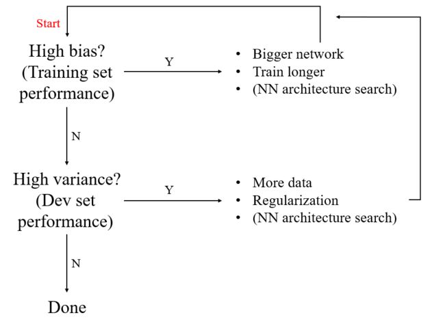
• In a word, training set performance represents bias problem, and dev set performance represents variance problem.

In the 2-dimensional case, we could draw the following graphs:

1.3 Basic recipe for machine learning

---

1.4 Regularization

---

Prevent over-fitting, and reduce the variance.

1) L2 Regularization (or Weight Decay) in neural network

• lambda is called the regularization parameter

• From the perspective of "weight decay", the expression of updating W^[l] could be rewritten as:

2) How does regularization prevent from over-fitting?

用下图简单说明。

当我们把正则化参数lambda设置得很小时，系统趋于没有正则化的情况，即右图的过度拟合（over-fitting）情况；

当我们把lambda设置得很大时，系统中的大部分节点权重极小，导致网络退化为一个简单的形式，类似左图中欠拟合（underfitting）的情况；

因此，存在一个lambda的中间值，使得系统落在中间图的情况。

因此我们要做的是寻找恰当的lambda，既能减小方差（variance），又能保持较小的偏置（bias）。

简单来说，正则化的作用就是使过度拟合的网络向线性的方向退化，以期减少过拟合的情况。

3) Dropout (随机失活) Regularization

Dropout Regularization: 在训练神经网络的过程中，对每一个样本，在每一层的运算间随机关闭掉（失活）一些节点。也就是说，对每个样本，它经过的网络都是原网络的一个随机产生的子网络

• keep-prob: The probability that a given hidden unit will be kept

• 下面给出一个Dropout Regularization的可能实现，被称为 Inverted Dropout （反向随机失活）。代码中仅用一个大网络的第3层的Dropout作为示范，其中变量a3即为a^[3]

# Illustrate with layer l = 3

keep_prob = 0.8

d3 = np.random.rand(a3.shape[0], a3.shape[1]) < keep_prob 
#matrix d3 of type bool，value false marks the nodes to be dropped out

a3 = np.multiply (a3, d3)       
# element-wise multiplication, true is converted to 1 while false is converted to 0

a3 /= keep_prob
# so that the dropped out nodes won't affect the expectation of a3

• 在测试时不要使用dropout，因为你并不希望测试时对一个输入给出的结果是随机的

• 每一层的 keep_prob 可以单独选取。权重矩阵较大的层，更有可能过度拟合，所以我们倾向于选择更小的 keep_prob（如0.5）；一般的层可以选择如0.7；完全不用担心过度拟合的小矩阵层，甚至可以选择1.0，即不使用随机失活。

• input layer 的keep_prob通常选择1

4) Other Regularization Methods

(For more detail, please watch the video.)

• Data augmentation 数据扩增

• Early stopping

1.5 Normalizing Input Features

---

Two steps

1. zero out the means (零均值化)

2. normalize the variances (归一化方差)

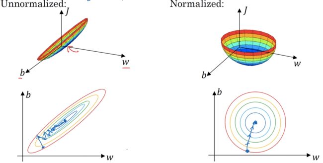
Why normalize inputs?

归一化输入的好处在于，代价函数更加均匀。因此我们不论选取怎样的学习率alpha，最终都能顺利到达最优点。

反之，如果输入没有归一化，则代价函数的图形如左图所示（以二维输入为例），则我们不得不选取很小的学习率alpha，以期在多轮迭代后不会错过最优点。

1.6 Vanishing / Exploding Gradients 梯度消失与梯度爆炸

---

• If the weights W is a little bit bigger than the identity matrix, then with a very deep network, the activations can explode;

• If the weights W is a little bit less than the identity, then in a very deep network, the activations will decrease exponentially.

• In summary, deep networks suffer from the problem of vanishing or exploding gradients.

• A partial solution to this is better or more careful choice of the random initialization for your neural network.

1.7 Weight Initialization for Deep Networks

---

• 思路：输入特征数越多，权重初始值越小。这样可以维持激活（activation）在维度增长时不会过大或过小。

• 在深度神经网络中的应用：

# weight matrix initialization
W[l] = np.random.randn() * np.sqrt(2/n[l-1])

# Here is some notes about the expression in the sqrt parenthesis
#
# if the activation function is ReLU, 
#    then you should use: np.sqrt(2/n[l-1])
#
# and if the activation function is tanh, 
#     then you should use np.sqrt(1/n[l-1]) or np.sqrt(2 / (n[l-1] + n[l]))

1.8 Gradient Checking 梯度检验

---

• 思路：根据导数的定义，可以用以下式子的结果逼近导数的值。

• 在深度神经网络中，这个思路被用来做梯度检验。

• 一些注意要点：
  • 不要在训练时使用梯度检验——只在调试时使用；
  • 使用梯度检验时需注意有没有正则化；
  • 梯度检验不能和随机失活一起使用；
  • 随机初始化的情形下，建议先训练一段时间后再引入梯度检验。

2 Optimization Algorithms

2.1 Mini-batch Gradient Descent

---

Notation

notation	name	explanation
(i)	round brackets	index of different training examples
[i]	square brackets	index of different layers of the neural network
{t}	curly brackets	index of different mini batches

• Batch gradient descent: process your whole training set at the same time
• Mini-batch gradient descent: process a single mini batch at the same time

Intuition

• Idea: Instead of applying gradient descent after processing the whole training set, we could use gradient descent after processing each mini batch.

• One epoch (一代) of training: a single pass through the training set, or processing all the mini batches once

• Advantage of mini batch gradient descent: one epoch allows you to take many gradient descent steps.

• When you are training on a large dataset, using mini-batch is much faster than using only batch.

Further Understanding

(Watch the whole fruitful video for more details.)

• If you choose 1 as your mini batch size, then your algorithm becomes stochastic gradient descent, which loses all the speedup from vectorization;
• If you choose m as your mini batch size, then your algorithm becomes batch gradient descent, which takes too much time for each iteration;
• Choose your mini batch size between 1 (too small) and m (too large). It would be better if you choose sizes such as 64 (2⁶), 128 (2⁷), 256 (2⁸), 512 (2⁹). Because the computer memory is binary.

2.2 Exponentially Weighted Average

---

• The effect of this exponentially weighted average is to take the approximate average on the past 1/(1-beta) data. This could be demonstrated by the following formula.

• Comparing to directly take average on the past data, this method runs much faster and saves memory.

Bias Correction

• 事实上，用上面给出的指数下降公式，得到的平均结果在前几天的值是不准确的。如上图所示，设置beta=0.98，用上面的公式得到的是紫色曲线。

• 引入Bias Correction，将预测值v_t变为下式，就得到了图中的绿色曲线。显然绿色曲线更好地平均了初始阶段的蓝色数据点。

• 机器学习中，有时人们不会引入Bias Correction。

2.3 Gradient Descent With Momentum

---

• 蓝色线条：普通的梯度下降算法，合适的学习率
• 紫色线条：普通的梯度下降算法，过高的学习率
• 红色线条：动量梯度下降法（Gradient Descent With Momentum）

Implementation

首先初始化矩阵 v_dW, v_db 为全0矩阵。

Gradient descent with momentum will almost always work better than the straightforward gradient descent without momentum.

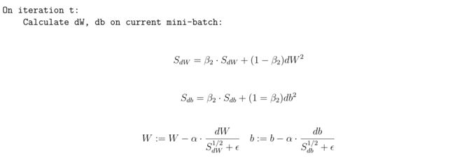
2.4 RMSprop Optimization Algorithm

---

RMS stands for "Root mean square".

• 思路：改变大的项除以一个大的值来变小；改变小的项除以一个小的值来变大。

• 好处：可以用更大的学习率而不用担心偏移过大。（其实好的优化下都可以用大一点的学习率）

Implementation

初始化 S_dW, S_db 为 零矩阵。

epsilon是防止分母为0引入的一个小值，可以选择如10e-8 。

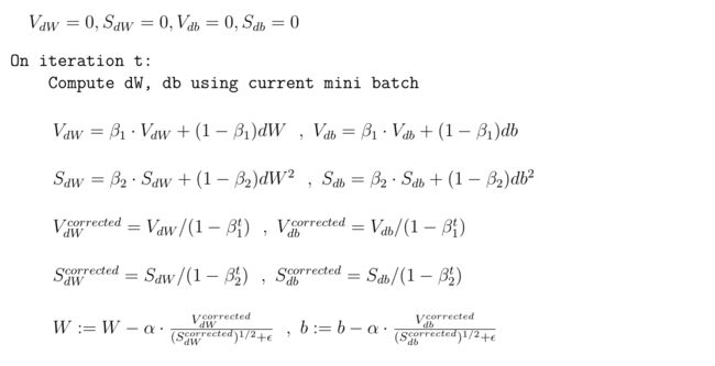
2.5 Adam Optimization Algorithm

---

Adam represents "Adaptive Moment Estimation".

Algorithm

Default Parameter Setting

2.6 Learning Rate Decay

---

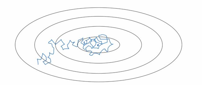
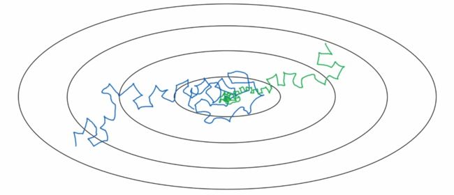
• 学习率不衰减的情况：不会精确地收敛，而是在最优值附近摆动

• 引入学习率衰减（绿线）：最终在最优值附近的极小区域波动

Implementation

• 3 simple methods:

• You could also use:
  • Discrete staircase
  • Manual decay

---

吴教授指出了深度学习优化算法的问题，不在于落入局部最优点。这是因为在高维条件下，出现局部最优的条件是所有维度的凹凸性一致，所以大部分梯度为0的点是鞍点（saddle）。

而优化算法真正的问题，在于平缓段（plateau）对学习效率的影响。当学习进入到平缓阶段时，就需要用好的优化算法离开平缓段。

3 Hyperparameter Tunning

3.1 Tuning Process

---

• Use random values: Don't use grid
• Take a coarse to fine scheme

#实现在对数坐标上的随机取样
r = -4 * np.random.rand()
alpha = 10**r

3.2 Batch Norm (BN)

---

归一化输出层的推广：每一层都进行归一化。

我们通常只需要在框架里直接使用BN就可以了，若想了解详细的原理和实现，请参考下面几个视频：

• Batch norm入门
• Batch norm在深度网络中的实现
• Batch norm原理分析
• 使用Batch norm后测试时的一些不同

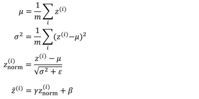
给出某一层的计算式：

参数beta和gamma需要用梯度下降来学习。值得一提的是，如果使用了BN，每一层的参数b可以省略了。因为无论加上了什么常数，在归一化时都会被减去。

• It limits the amount to which updating the parameters in the earlier layers can effect the distribution of values that a later layer sees and learns on.

• Batch norm reduces the problem of the input values changing, it really causes these values to become more stable.

• Batch norm adds some noise to each hidden layer's activations. And so similar to dropout, batch norm therefore has a slight regularization effect.

3.3 Softmax Regression

---

• Softmax regression is a generalization of logistic regression. Softmax regression could classify C (C > 2) classes.

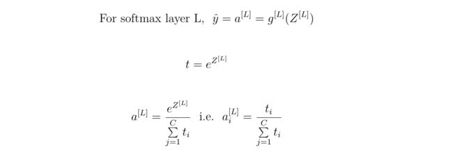
Math of the Softmax Layer

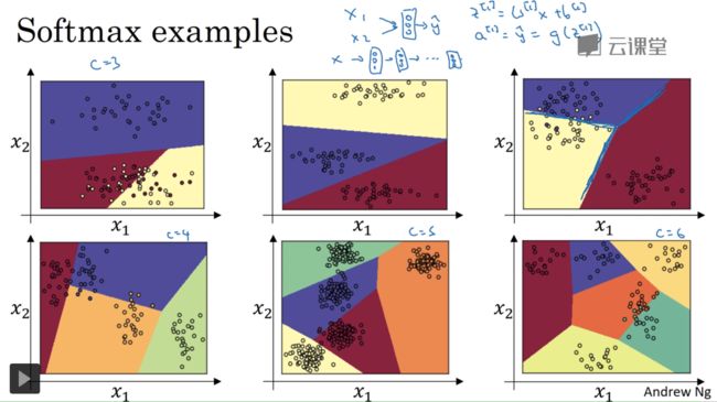
Softmax Examples

• Note that in this example, the classifier has no hidden layer, but only one softmax layer.

Training a Softmax Classifier

And for the gradient descent, the first expression should be:

3.4 Deep Learning Frameworks

---