【深度学习-9】用TensorFlow构建卷积神经网络（一）

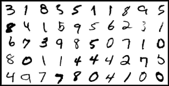
在具备了一定的基础知识后，我们终于可以开始动手构建卷积神经网络了。根据TensorFlow官网上的教程，A Guide to TF Layers: Building a Convolutional Neural Network，我们先来学习怎样使用TF中的layers模块构建一个简单的卷积神经网络来识别手写数字（handwritten digits）。我们用到的数据集（手写数字0-9的黑白图片）来自MNIST（ http://yan.lecun.com ），总共包括60000个训练数据和10000个测试数据，图片的大小为28×28像素。教程的完整代码(cnn_mnist.py)可以在github上找到。

mnist.png

我们首先尝试构建一个简单的卷积神经网络，它的结构如下：

1. Input Layer
2. Convolutional Layer #1：32个5×5的filter，使用ReLU激活函数
3. Pooling Layer #1：2×2的filter做max pooling，步长为2
4. Convolutional Layer #2：64个5×5的filter，使用ReLU激活函数
5. Pooling Layer #2：2×2的filter做max pooling，步长为2
6. Dense Layer #1：1024个神经元，使用ReLU激活函数，dropout率0.4 (为了避免过拟合，在训练的时候，40%的神经元会被随机去掉)
7. Dense Layer #2 (Logits Layer)：10个神经元，每个神经元对应一个类别（0-9）

我们在cnn_mnist.py的代码中可以看到，构建CNN模型的任务是通过cnn_model_fn函数来实现的：

def cnn_model_fun(feature, labels, mode):
    """Model function for CNN."""
    ......

在这个函数中，我们用TensorFlow的layers模块一步步构建卷积神经网络。主要用3个method：conv2d()，max_pooling2d()和dense()来分别创建Convolutional Layer，Pooling Layer和Dense Layer。除此之外，我们还要定义loss function，配置training op，并生成预测值。

下面将逐段分析cnn_model_fn函数的代码。

Input Layer

# Input Layer
# Reshape X to 4-D tensor: [batch_size, width, height, channels]
# MNIST images are 28x28 pixels, and have one color channel
input_layer = tf.reshape(feature, [-1, 28, 28, 1])

输入层的tensor（input_layer）一共有4个dimension，分别是：[ batch_size, image_width, image_height, channels]
batch_size：每次训练使用的训练集的子集的大小
image_width：图像的宽
image_height：图像的高
channels：彩色图像值为3，黑白图像值为1
我们将大小为28×28的黑白照片通过feature参数传递进来（每个值代表一个像素），然后reshape成4-D的输入层tensor。batch_size取-1表示该值是在其他3个值不变的情况下，根据feature的长度动态计算出的。这样做的好处是可以把batch_size作为一个可以调的hyperparameter。

Convolutional Layer #1

# Computes 32 features using a 5x5 filter with ReLU activation.
# Padding is added to preserve width and height.
# Input Tensor Shape: [batch_size, 28, 28, 1]
# Output Tensor Shape: [batch_size, 28, 28, 32]
conv1 = tf.layers.conv2d(
    inputs=input_layer,
    filters=32,
    kernel_size=[5, 5],
    padding='same',
    activation=tf.nn.relu)

我们使用conv2d来创建卷积层。在这一层中，我们需要32个5×5的filter，并且使用ReLU激活函数。padding=‘same’的意思是：通过zero-padding的办法，保证input和output tensor的大小一致。其他参数都很好理解。输出的tensor的shape为[batch_size, 28, 28, 32]，现在的channel数为32，每个channel对应一个filter的输出。

Pooling Layer #1

# First max pooling layer with a 2x2 filter and stride of 2
# Input Tensor Shape: [batch_size, 28, 28, 32]
# Output Tensor Shape: [batch_size, 14, 14, 32]
pool1 = tf.layers.max_pooling2d(inputs=conv1, pool_size=[2, 2], strides=2)

我们使用max_pooling2d来创建pooling层。在这一层中，我们需要2×2的filter做max pooling，步长为2。输出的tensor的shape为[batch_size, 14, 14, 32]。

Convolutional Layer #2 and Pooling Layer #2

根据同样的方法创建，代码如下：

# Convolutional Layer #2
# Computes 64 features using a 5x5 filter.
# Padding is added to preserve width and height.
# Input Tensor Shape: [batch_size, 14, 14, 32]
# Output Tensor Shape: [batch_size, 14, 14, 64]
conv2 = tf.layers.conv2d(
    inputs=pool1,
    filters=64,
    kernel_size=[5, 5],
    padding='same',
    activation=tf.nn.relu)

# Pooling Layer #2
# Second max pooling layer with a 2x2 filter and stride of 2
# Input Tensor Shape: [batch_size, 14, 14, 64]
# Output Tensor Shape: [batch_size, 7, 7, 64]
pool2 = tf.layers.max_pooling2d(inputs=conv2, pool_size=[2, 2], strides=2)

conv2的shape为[batch_size, 14, 14, 64]，pool2的shape为[batch_size, 7, 7, 64]

Dense Layer

# Flatten tensor into a batch of vectors
# Input Tensor Shape: [batch_size, 7, 7, 64]
# Output Tensor Shape: [batch_size, 7 * 7 * 64]
pool2_flat = tf.reshape(pool2, [-1, 7 * 7 * 64])

在构建dense层之前，我们先把pool2的dimension从4变成2，也就是把shape改为[batch_size, 7 × 7 × 64]。

# Dense Layer
# Densely connected layer with 1024 neurons
# Input Tensor Shape: [batch_size, 7 * 7 * 64]
# Output Tensor Shape: [batch_size, 1024]
dense = tf.layers.dense(inputs=pool2_flat, units=1024, activation=tf.nn.relu)

接下来我们用dense方法来创建dense层，一共有1024个神经元，并且使用ReLU激活函数。dense的shape为[batch_size, 1024]。

然后对dense层使用dropout regularization：

# Add dropout operation; 0.6 probability that element will be kept
dropout = tf.layers.dropout(inputs=dense, rate=0.4, training=mode == learn.ModeKeys.TRAIN)

mode指的是模型运行的模式，有三种：TRAIN，EVAL和INFER。当mode为TRAIN的时候，training参数为True，dropout才能执行。dropout tensor的shape为[batch_size, 1024]

Logits Layer

# Logits layer
# Input Tensor Shape: [batch_size, 1024]
# Output Tensor Shape: [batch_size, 10]
logits = tf.layers.dense(inputs=dropout, units=10)

这是神经网络的最后一层，返回的是我们预测的原始值。用10个神经元对应0-9十个数，激活函数使用的是默认值（线性激活函数）。logits的shape是[batch_size, 10]。

Calculate Loss

在训练（TRAIN）和评估（EVAL）的时候，我们需要定义一个损失函数（loss function）来衡量模型的预测值和真实值之间的距离。对于多元分类问题，我们通常使用cross entropy来作为loss。

loss = None
train_op = None
# Calculate loss for both TRAIN and EVAL modes
if mode != learn.ModeKeys.INFER:
    onehot_labels = tf.one_hot(indices=tf.cast(labels, tf.int32), depth=10)
    loss = tf.losses.softmax_cross_entropy(
        onehot_lables=onehot_lables, logits=logits)

为了计算cross-entropy，我们首先要用tf.one_hot函数把图像的labels（[1,3,4,9,...]）转成one-hot encoding格式。tf.losses.softmax_cross_entropy函数先在logits上使用softmax激活函数（得到每个class的概率），然后计算onehot_lables和logits之间的cross-entropy。

Configure the Training Op

# Configure the Training Op (for TRAIN mode)
if mode == learn.ModeKeys.TRAIN:
    train_op = tf.contrib.layers.optimize_loss(
        loss=loss,
        global_step=tf.contrib.framework.get_global_step(),
        learning_rate=0.001,
        optimizer="SGD")

在定义了loss后，我们要告诉TF如何在训练中优化这个loss。我们使用的是tf.contrib.layers.optimize_loss函数，学习速率设为0.001，优化算法是随机梯度下降（Stochastic Gradient Descent，SGD）。

Generate Prediction

# Generate Predictions
predictions = {
    "classes": tf.argmax(input=logits, axis=1),
    "probabilities": tf.nn.softmax(logits, name="softmax_tensor")
}

Logits Layer 返回的logits是预测的原始值，我们需要将其转换成预测的类别（classes）和概率（probabilities）。对于每个example来说，我们预测的类别就是原始值最高的那个类，可以用tf.argmax函数来获得。在logits上使用softmax激活函数tf.nn.softmax可以得到每个类的概率。

ModelFnOps object

# Return a ModelFnOps object
return model_fn_lib.ModelFnOps(mode=mode, predictions=predictions, loss=loss, train_op=train_op)

最后，我们将得到的predictions，loss，train_op和mode参数一起放到ModelFnOps对象中并作为cnn_model_fun函数的返回值。

创建完CNN模型函数cnn_model_fun后，我们就可以开始对模型进行训练和评估。这部分代码在main()函数中：

def main(unused_argv):
    ......

下面将逐段分析main函数的代码。

Loading Training and Test Data

# Load training and eval data
mnist = learn.datasets.load_dataset("mnist")
train_data = mnist.train.images  # Returns np.array
train_labels = np.asarray(mnist.train.labels, dtype=np.int32)
eval_data = mnist.test.images  # Returns np.array
eval_labels = np.asarray(mnist.test.labels, dtype=np.int32)

TF会自动下载MNIST数据集，并将训练集（train）和测试集（eval）的原始像素值（data）和标签（labels）存放在numpy arrays中。

Create the Estimator

# Create the Estimator
mnist_classifier = learn.Estimator(model_fn=cnn_model_fn, model_dir="/tmp/mnist_convnet_model")

Estimator是TF对模型进行训练（training），评估（evaluation）和推断（inference）所用的类。model_dir参数用来指定模型数据和检查点（checkpoints）的存放路径。

Set Up a Logging Hook

# Set up logging for predictions
# Log the values in the "Softmax" tensor with label "probabilities"
tensors_to_log = {"probabilities": "softmax_tensor"}
logging_hook = tf.train.LoggingTensorHook(tensors=tensors_to_log, every_n_iter=50)

由于CNN的训练时间比较长，我们需要TF输出logging来跟踪训练的进程。在上面的例子中，我们使用tf.train.LoggingTensorHook，要求每训练50次的时候输出预测的概率值。

Train the Model

# Train the model
mnist_classifier.fit(
    x=train_data,
    y=train_labels,
    batch_size=100,
    steps=20000,
    monitors=[logging_hook])

我们现在可以用mnist_classifier的fit()方法进行模型的训练。feature和labels分别传递给x和y，batch_size=100的意思是模型每次（step）在由100个样本组成的小训练集上进行训练，steps=20000表示模型总共训练20000次。将logging_hook传递给monitors参数可以在训练的时候输出我们指定的logging。

Evaluate the Model

训练结束后，我们要对模型的准确率进行评估。首先用MetricSpec设定准确性的度量标准（accuracy metric）：

# Configure the accuracy metric for evaluation
metrics = {
    "accuracy":
        learn.MetricSpec(
            metric_fn=tf.metrics.accuracy, prediction_key="classes"),
}

然后将评估数据集（eval_data和eval_labels）和metric传给mnist_classifier的evaluate方法，得到最终的评估结果。

# Evaluate the model and print results
eval_results = mnist_classifier.evaluate(x=eval_data, y=eval_labels, metrics=metrics)
print(eval_results)

Run the Model

运行cnn_mnist.py脚本，训练模型并得到最终的准确率。

accuracy.png

我算出的准确率为96.9%，比教程中的略低（97.3%）。

qrcode.jpg