测试设备:iPad Air 2, iOS 9.2。
1、透视渲染一个3维图表
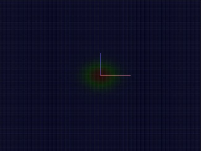
上一章iOS OpenGL ES 3.0 数据可视化 2:平面数据可视化最后绘制了平面热度图,虽没显式设置顶点着色器的正交投影矩阵,实际默认应用了正交投影,本节将它改成3维图形,运行效果如下所示。

1.1、实现代码与分析
修改上章代码,加上4x4矩阵定义、顶点着色器加上MVP矩阵运算等内容。
#import

@interface MyGLView : UIView

@end

GLfloat ratio = 0.0f;
GLuint renderbuffer;
GLuint framebuffer;
GLuint program;
GLint renderbufferWidth, renderbufferHeight;

typedef struct {
    GLfloat x, y, z; //position
    GLfloat r, g, b, a; //color and alpha channels
} Vertex;

typedef struct {
    GLfloat x, y, z;
} Data;

typedef float vec4[4];
typedef vec4 mat4x4[4];

@interface MyGLView () {
    CAEAGLLayer *glLayer;
    EAGLContext *context;
}

@end

@implementation MyGLView

+ (Class)layerClass {
    return [CAEAGLLayer class];
}

- (void)layoutSubviews {
    [super layoutSubviews];

    glLayer = (CAEAGLLayer *) self.layer;
    glLayer.contentsScale = [UIScreen mainScreen].scale;
    glLayer.drawableProperties = @{
                                   kEAGLDrawablePropertyRetainedBacking : @(FALSE),
                                   kEAGLDrawablePropertyColorFormat : kEAGLColorFormatRGBA8};

    context = [[EAGLContext alloc] initWithAPI:kEAGLRenderingAPIOpenGLES3];
    [EAGLContext setCurrentContext:context];

    glGenRenderbuffers(1, &renderbuffer);
    glBindRenderbuffer(GL_RENDERBUFFER, renderbuffer);
    [context renderbufferStorage:GL_RENDERBUFFER fromDrawable:glLayer];

    glGetRenderbufferParameteriv(GL_RENDERBUFFER, GL_RENDERBUFFER_WIDTH, &renderbufferWidth);
    glGetRenderbufferParameteriv(GL_RENDERBUFFER, GL_RENDERBUFFER_HEIGHT, &renderbufferHeight);
    NSLog(@"(renderbufferWidth, renderbufferHeight) = (%d, %d)", renderbufferWidth, renderbufferHeight);

    glGenFramebuffers(1, &framebuffer);
    glBindFramebuffer(GL_FRAMEBUFFER, framebuffer);
    glFramebufferRenderbuffer(GL_FRAMEBUFFER, GL_COLOR_ATTACHMENT0, GL_RENDERBUFFER, renderbuffer);

    char *vertexShaderContent =
        "#version 300 es \n"
        "layout(location = 0) in vec4 position; "
        "layout(location = 2) in vec4 point_color; "
        "uniform mat4 projection_matrix; "
        "uniform mat4 model_matrix; "
        "out vec4 v_point_color; "
        "void main() { "
            "gl_Position = projection_matrix * model_matrix * position; "
            "gl_PointSize = 3.0;"
            "v_point_color = point_color; "
        "}";
    GLuint vertexShader = compileShader(vertexShaderContent, GL_VERTEX_SHADER);

    char *fragmentShaderContent =
        "#version 300 es \n"
        "precision highp float; "
        "in vec4 v_point_color; "
        "uniform bool is_sprite; "
        "out vec4 fragColor; "
            "void main() { "
            "if (is_sprite) {"
                "if(length(gl_PointCoord-vec2(0.5)) > 0.5) discard;"
            "}"
            "else "
                "fragColor = v_point_color;"
        "}";
    GLuint fragmentShader = compileShader(fragmentShaderContent, GL_FRAGMENT_SHADER);

    program = glCreateProgram();
    glAttachShader(program, vertexShader);
    glAttachShader(program, fragmentShader);

    glLinkProgram(program);
    GLint linkStatus;
    glGetProgramiv(program, GL_LINK_STATUS, &linkStatus);
    if (linkStatus == GL_FALSE) {
        GLint infoLength;
        glGetProgramiv(program, GL_INFO_LOG_LENGTH, &infoLength);
        if (infoLength > 0) {
            GLchar *infoLog = malloc(sizeof(GLchar) * infoLength);
            glGetProgramInfoLog(program, infoLength, NULL, infoLog);
            printf("%s\n", infoLog);
            free(infoLog);
        }
    }

    glUseProgram(program);

    glEnable(GL_BLEND);
    glBlendFunc(GL_SRC_ALPHA, GL_ONE_MINUS_SRC_ALPHA);

    glClearColor(0, 0, 0, 1.0);
    glClear(GL_COLOR_BUFFER_BIT);

    glViewport(0, 0, renderbufferWidth, renderbufferHeight);

    ratio = renderbufferWidth * 1.0 / renderbufferHeight;

    CADisplayLink *link = [CADisplayLink displayLinkWithTarget:self selector:@selector(update:)];
    [link addToRunLoop:[NSRunLoop currentRunLoop] forMode:NSRunLoopCommonModes];
}

- (void)update:(CADisplayLink *)link {
    glClearColor(0, 0, 0, 1.0);
    glClear(GL_COLOR_BUFFER_BIT);

    draw3DGaussion(renderbufferWidth, renderbufferHeight);

    [context presentRenderbuffer:GL_RENDERBUFFER];
}
1.1.1、设置透视投影
原书对透视投影的说明如下:
Rendering a 3D scene is similar to taking a photograph with a digital camera in the real world. The steps that are taken to create a photograph can also be applied in OpenGL.
For example, you can move the camera from one position to another and adjust the viewpoint freely in space, which is known as viewing transformation. You can also adjust the position and orientation of the the object of interest in the scene. However, unlike in the real world, in the virtual world you can position the object at any orientation freely without any physical constraints, termed as modeling transformation. Finally, we can exchange camera lenses to adjust the zoom and create different perspectives the process is called projection transformation.
When you take a photo applying the viewing and modeling transformation, the digital camera takes the information and creates an image on your screen. This process is called rasterization.
These sets of matrices—encompassing the viewing transformation, modeling transformation, and projection transformation are the fundamental elements we can adjust at runtime, which allows us to create an interactive and dynamic rendering of the scene. To get started, we will first look into the setup of the camera matrix, and how we can create a scene with different perspectives.
更多坐标空间变换描述可参考红书、蓝书等,下图示意了透视投影的参数。

整合glfw中的代码,也可按OpenGL ES 1.0的文档自行实现相关的矩阵运算,反正构造出来的矩阵就是行优先或列优先存储两种形式。
void draw3DGaussion(int renderbufferWidth, int renderbufferHeight) {
    const float fovY = 60.0f;
    const float front = .1f;
    const float back = 128.f;

    /* Compute the projection matrix */
    mat4x4 projectionMatrix;
    mat4x4_identity(projectionMatrix);
    mat4x4_perspective(projectionMatrix_perspective, fovY, ratio, front, back);
    int projection_matrix_location = glGetUniformLocation(program, "projection_matrix");
    glUniformMatrix4fv(projection_matrix_location, 1, GL_FALSE, projectionMatrix);

    GLfloat alpha = 210.0f, beta = -70.0f, zoom = 2.0f;
    float sigma = 0.1f;
    float sign = 1.0f;
    float step_size = 0.01f;

    mat4x4 modelMatrix;
    mat4x4_translate(modelMatrix, 0.0, 0, -2.7);
    // rotate by beta degrees around the x-axis
    mat4x4_rotate_X(modelMatrix, modelMatrix, beta);
    // rotate by alpha degrees around the z-axis
    mat4x4_rotate_Z(modelMatrix, modelMatrix, alpha);
    int model_matrix_location = glGetUniformLocation(program, "model_matrix");
    glUniformMatrix4fv(model_matrix_location, 1, GL_FALSE, modelMatrix);

    drawOrigin();
    sigma = sigma + sign * step_size;
    if (sigma > 1.0f) {
        sign = -1.0f;
    }
    if (sigma < 0.1) {
        sign = 1.0f;
    }
    gaussianDemo(sigma);
}
原书代码为gluPerspective(fovY, ratio, front, back);,gluPerspective接受角度值,其形式如下所示,在此对应mat4x4_perspective函数。
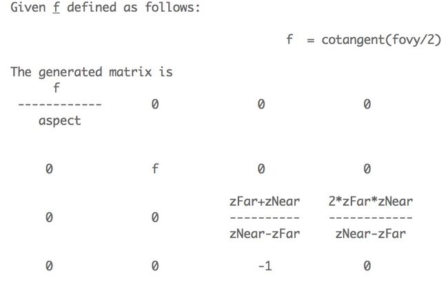
The aspect: ratio is the ratio of x (width) to y (height).
对比glTranslate函数的定义,可知,OpenGL ES 1.0使用向量右乘计算,即matrix4x4 * vec4 = new vec4。
而glfw定义的平移矩阵为左乘,即vec4 * matrix4x4 = new vec4,反映到着色器是gl_Position = projection_matrix * model_matrix * position;。有关矩阵左、右乘问题在后续内容再讨论。
static inline void mat4x4_translate(mat4x4 T, float x, float y, float z) {
   mat4x4_identity(T);
   T[3][0] = x;
   T[3][1] = y;
   T[3][2] = z;
}
观察mat4x4_translate的实现,正好是glTranslate的转置矩阵。同理,glfw其他矩阵的运算也是左乘。
static inline void mat4x4_perspective(mat4x4 m, float y_fov_in_degrees, float aspect, float n, float f) {
    /* NOTE: Degrees are an unhandy unit to work with.
     * linmath.h uses radians for everything! */
    const float angle_in_radians = (float) (y_fov_in_degrees * M_PI / 180.0);
    float const a = 1.f / (float) tan(angle_in_radians / 2.f);

    m[0][0] = a / aspect;
    m[0][1] = 0.f;
    m[0][2] = 0.f;
    m[0][3] = 0.f;

    m[1][0] = 0.f;
    m[1][1] = a;
    m[1][2] = 0.f;
    m[1][3] = 0.f;

    m[2][0] = 0.f;
    m[2][1] = 0.f;
    m[2][2] = -((f + n) / (f - n));
    m[2][3] = -1.f;

    m[3][0] = 0.f;
    m[3][1] = 0.f;
    m[3][2] = -((2.f * f * n) / (f - n));
    m[3][3] = 0.f;
}
gluPerspective与glFrustum生成的矩阵是相等的,同理,mat4x4_perspective与mat4x4_frustum函数构造出来的矩阵也是相等的,二者可随时替换。值得注意的是,glfw的矩阵运算接口都使用弧度,调用前需做单位转换,在此,我把转换处理放在函数体,省去每次调用前的预处理。下面给出OpenGL ES 1.0中glFrustum的定义及对应mat4x4_frustum函数。

static inline void mat4x4_frustum(mat4x4 M, float l, float r, float b, float t, float n, float f) {
    M[0][0] = 2.f * n / (r - l);
    M[0][1] = M[0][2] = M[0][3] = 0.f;

    M[1][1] = 2.f * n / (t - b);
    M[1][0] = M[1][2] = M[1][3] = 0.f;

    M[2][0] = (r + l) / (r - l);
    M[2][1] = (t + b) / (t - b);
    M[2][2] = -(f + n) / (f - n);
    M[2][3] = -1.f;

    M[3][2] = -2.f * (f * n) / (f - n);
    M[3][0] = M[3][1] = M[3][3] = 0.f;
}
mat4x4_identity将矩阵重置为单位矩阵,定义如下。
static inline void mat4x4_identity(mat4x4 M) {
    int i, j;
    for (i = 0; i < 4; ++i)
        for (j = 0; j < 4; ++j)
            M[i][j] = i == j ? 1.f : 0.f;
}
平移矩阵mat4x4_translate定义如下。
static inline void mat4x4_translate(mat4x4 T, float x, float y, float z) {
    mat4x4_identity(T);
    T[3][0] = x;
    T[3][1] = y;
    T[3][2] = z;
}
mat4x4_translate(modelMatrix, 0.0, 0.0, -2.0);得到如下操作结果。
1,   0,   0,   0
0,   1,   0,   0
0,   0,   1,   0
0,   0,  -2,   1
绕X、Y、Z轴的旋转矩阵容易推导,绕任意轴旋转则略为麻烦,需分别映射到X、Y、Z平面、平移、旋转,再作反操作,共7个矩阵相乘,结果矩阵如下所示。

本节目前只使用mat4x4_rotate_X绕X轴旋转、mat4x4_rotate_Z绕Z轴旋转矩阵函数。
static inline void mat4x4_rotate_X(mat4x4 Q, mat4x4 M, float angle_in_degrees) {
    const float angle_in_radians = (float) (angle_in_degrees * M_PI / 180.0);
    float s = sinf(angle_in_radians);
    float c = cosf(angle_in_radians);
    mat4x4 R = {
        {1.f, 0.f, 0.f, 0.f},
        {0.f,   c,   s, 0.f},
        {0.f,  -s,   c, 0.f},
        {0.f, 0.f, 0.f, 1.f}
    };
    mat4x4_mul(Q, M, R);
}

static inline void mat4x4_rotate_Z(mat4x4 Q, mat4x4 M, float angle_in_degrees) {
    const float angle_in_radians = (float) (angle_in_degrees * M_PI / 180.0);
    float s = sinf(angle_in_radians);
    float c = cosf(angle_in_radians);
    mat4x4 R = {
        {   c,   s, 0.f, 0.f},
        {  -s,   c, 0.f, 0.f},
        { 0.f, 0.f, 1.f, 0.f},
        { 0.f, 0.f, 0.f, 1.f}
    };
    mat4x4_mul(Q, M, R);
}

static inline void mat4x4_mul(mat4x4 M, mat4x4 a, mat4x4 b) {
    mat4x4 temp;
    int k, r, c;
    for (c = 0; c < 4; ++c)
        for (r = 0; r < 4; ++r) {
            temp[c][r] = 0.f;
            for (k = 0; k < 4; ++k)
                temp[c][r] += a[k][r] * b[c][k];
        }
    mat4x4_dup(M, temp);
}

static inline void mat4x4_dup(mat4x4 M, mat4x4 N) {
    int i, j;
    for (i = 0; i < 4; ++i)
        for (j = 0; j < 4; ++j)
            M[i][j] = N[i][j];
}
1.1.2、绘制坐标轴
void drawOrigin() {
    float transparency = 0.5f;
    // draw a red line for the x-axis
    {
        Vertex start = {0.0f, 0.0f, 0.0f,
            1.0f, 0.0f, 0.0f, transparency};
        Vertex end = {0.3f, 0.0f, 0.0f,
            1.0f, 0.0f, 0.0f, transparency};
        drawLineSegment(start, end, 4.0f);
    }

    // draw a green line for the y-axis
    {
        Vertex start = {0.0f, 0.0f, 0.0f,
            0.0f, 1.0f, 0.0f, transparency};
        Vertex end = {0.0f, 0.0f, 0.3f,
            0.0f, 1.0f, 0.0f, transparency};
        drawLineSegment(start, end, 4.0f);
    }
    // draw a blue line for the z-axis
    {
        Vertex start = {0.0f, 0.0f, 0.0f,
            0.0f, 0.0f, 1.0f, transparency};
        Vertex end = {0.0f, 0.3f, 0.0f,
            0.0f, 0.0f, 1.0f, transparency};
        drawLineSegment(start, end, 4.0f);
    }
}
简单起见,我在着色器中硬编码点精灵的大小gl_PointSize = 3.0;。
1.1.3、修改gaussianDemo函数
生成的点阵数量降低为400 x 400,同时幅度A增大10倍const float sigma_const = 10.0f * (sigma2 * 2.0f * (float) M_PI);,优化了循环中的sigma平方计算。
void gaussianDemo(float sigma) {
    const int grid_x = 400;
    const int grid_y = 400;
    const int num_points = grid_x * grid_y;
    Data *data = (Data *) malloc(sizeof(Data) * num_points);
    int data_counter = 0;

    // standard deviation
    const float sigma2 = sigma * sigma;
    // amplitude
    const float sigma_const = 10.0f * (sigma2 * 2.0f * (float) M_PI);

    for (float x = -grid_x / 2.0f; x < grid_x / 2.0f; x += 1.0f) {
        for (float y = -grid_y / 2.0f; y < grid_y / 2.0f; y += 1.0f) {
            float x_data = 2.0f * x / grid_x;
            float y_data = 2.0f * y / grid_y;
            // Set the mean to 0
            // compute the height z based on a 2D Gaussian function.
            float z_data = exp(-0.5f * (x_data * x_data) / (sigma2)
                    - 0.5f * (y_data * y_data) / (sigma2)) / sigma_const;
            data[data_counter].x = x_data;
            data[data_counter].y = y_data;
            data[data_counter].z = z_data;
            data_counter++;
        }
    }
    // visualize the result using a 2D heat map
    draw2DHeatMap(data, num_points);
    free(data);
}
1.1.4、修改draw2DHeatMap函数
修改内容是,使用z分量和透明度。
void draw2DHeatMap(const Data *data, int num_points) {
    float transparency = 0.25f;

    // locate the maximum and minimum values in the dataset
    float max_value = -999.9f;
    float min_value = 999.9f;
    for (int i = 0; i < num_points; i++) {
        const Data d = data[i];
        if (d.z > max_value) {
            max_value = d.z;
        }
        if (d.z < min_value) {
            min_value = d.z;
        }
    }
    const float halfmax = (max_value + min_value) / 2;

    // display the result
    Vertex *points = malloc(num_points * sizeof(Vertex));
    for (int i = 0; i < num_points; i++) {
        const Data d = data[i];
        float value = d.z;
        float b = 1.0f - value / halfmax;
        float r = value / halfmax - 1.0f;
        if (b < 0) {
            b = 0;
        }
        if (r < 0) {
            r = 0;
        }
        float g = 1.0f - b - r;
        Vertex curPoint = {d.x, d.y, d.z,
                r, g, b, transparency};
        points[i] = curPoint;
    }

    GLuint dataBuffer;
    glGenBuffers(1, &dataBuffer);
    glBindBuffer(GL_ARRAY_BUFFER, dataBuffer);
    glBufferData(GL_ARRAY_BUFFER, num_points * sizeof(Vertex), points, GL_STATIC_DRAW);

    glEnableVertexAttribArray(0);
    glVertexAttribPointer(0, 3, GL_FLOAT, GL_FALSE, sizeof(Vertex)/* 每份完整数据的,所以偏移整个结构体 */, NULL);

    glEnableVertexAttribArray(2);
    glVertexAttribPointer(2, 4, GL_FLOAT, GL_FALSE, sizeof(Vertex), (GLvoid *) offsetof(Vertex, r)/* 结构体内部数据的偏移 */);

    glDrawArrays(GL_POINTS, 0, num_points);

    glDisableVertexAttribArray(0);
    glDisableVertexAttribArray(1);
    glDisableVertexAttribArray(2);

    glDeleteBuffers(1, &dataBuffer);

    free(points);
}
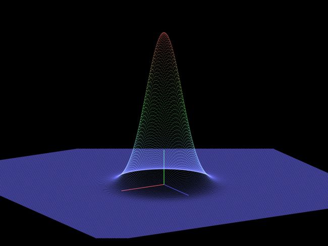
现在,运行程序可得到一个比原书效果差很多的图。
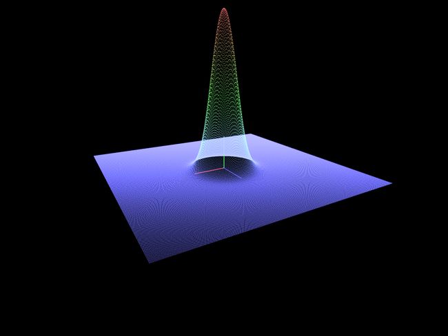
加上4倍线性多重采样后,底面点阵略有改善。
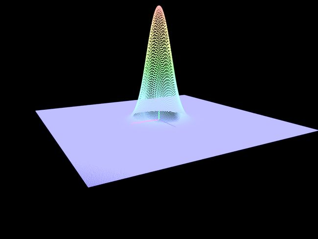
在4倍线性多重采样基础上改变混合方式为GL_ONE得到如下效果。
1.2、再讨矩阵定义与上传
目前矩阵定义为二维数组。
typedef float vec4[4];
typedef vec4 mat4x4[4];
相应的上传矩阵函数为glUniformMatrix4fv(model_matrix_location, 1 /* 矩阵个数 */, GL_FALSE, modelMatrix);,二维数组可正常上传。有些项目使用一维数组定义矩阵,如下所示,其上传方式和二维数组定义的矩阵是相同的。
static GLfloat modelview_matrix[16] = {
    1.0f, 0.0f, 0.0f, 0.0f,
    0.0f, 1.0f, 0.0f, 0.0f,
    0.0f, 0.0f, 1.0f, 0.0f,
    0.0f, 0.0f, 0.0f, 1.0f
};
1.3、再讨论矩阵的行、列优先存储
1.3.1、二维平面使用3x1或1x3向量的原因
以二维平面坐标点(x, y)为例,要平移至(x1, y1),2x2变换矩阵无法实现。比如,(1, 3)要平移到(5, 7),计算过程为
(1, 3) * 1 0 = (1, 3) != (5, 7)
         0 1
可见,2x2矩阵无法表达平移结果。改成3x3变换矩阵,则
(1, 3, 1)  *  1 0 0 = (5, 7, 1)
              0 1 0
              4 4 1
三维空间使用4x1或1x4向量也是相同原因。
1.3.2、行、列优先存储在运算时的区别
以glfw 3.2为例,框架使用行向量(行矩阵),(x, y, z, w) x (4x4变换矩阵) = (x', y', z', w')行向量,验证如下:
mat4x4 modelMatrix;
mat4x4_translate(modelMatrix, 0.0, 0.0, -2.0);
// 操作结果:
1,   0,   0,   0
0,   1,   0,   0
0,   0,   1,   0
0,   0,  -2,   1
若是列向量,则4x4平移矩阵应该是
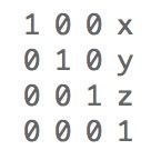
1,   0,   0,   a
0,   1,   0,   b
0,   0,   1,   c
0,   0,   0,   1
X轴上的点(1, 0, 0, 1)在Y轴上平移10个单位表示为(4x4平移矩阵) x (1, 0, 0, 1) = 结果矩阵。
1,   0,   0,   0
0,   1,   0,   10
0,   0,   1,   0
0,   0,   0,   1
现在验证glfw构造的旋转矩阵。绕X轴旋转的矩阵如下所示:
float s = sinf(angle);
float c = cosf(angle);
mat4x4 R = {
    {1.f, 0.f, 0.f, 0.f},
    {0.f,   c,   s, 0.f},
    {0.f,  -s,   c, 0.f},
    {0.f, 0.f, 0.f, 1.f}
};
那么,绕X轴旋转45度、直接传递45.0f给mat4x4_rotate_X()的结果为
1,                        0,                        0,                        0
0,               0.52532202,               0.85090351,                        0
0,               -0.8509035,               0.52532202,                        0
0,                        0,                        0,                        1
显然,cosf(45°)不等于0.52532202,而是0.7071067,需要把角度转换成弧度。
const float angle_in_radians = (float) (angle_in_degrees * M_PI / 180.0);
float s = sinf(angle_in_radians);
float c = cosf(angle_in_radians);
mat4x4 R = {
    {1.f, 0.f, 0.f, 0.f},
    {0.f,   c,   s, 0.f},
    {0.f,  -s,   c, 0.f},
    {0.f, 0.f, 0.f, 1.f}
};
参考:
OpenGL Data Visualization Cookbook, Raymond C. H. Lo. Chapter 3: Interactive 3D Data Visualization